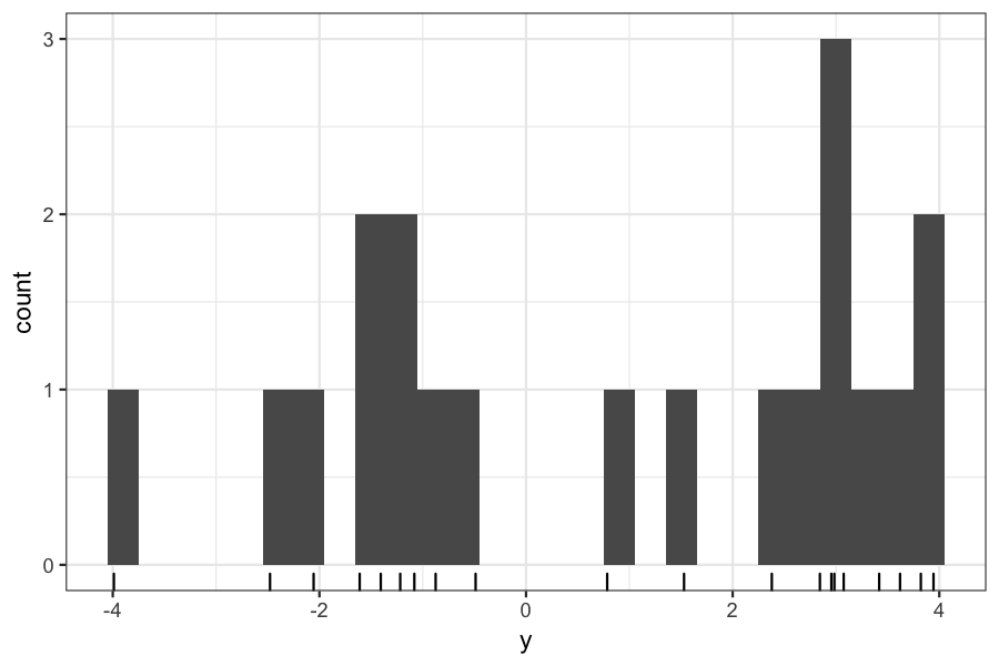
For example: Clustering with normal mixtures
Suppose we have a set of points measured on one variable.
We think that they come from two clusters, and we want to find the centers of those clusters.

Agenda today
Last day of optimization section
The EM algorithm
Reading: Lang Chapter 10
Goal, as usual: Maximize a likelihood
We've seen how we can do this in convex problems
EM is for the non-convex case
Particularly useful problems with "hidden data" or "missing data"
The idea behind EM:
There are some likelihoods that would be easy to maximize if we just had a littel bit of extra data
We can guess at what the missing data should be and find the parameters that maximize the likelihood based on our guess.
We then alternate between guessing at the missing data based on the current parameter estimates and estimating the parameters based on the guesses at the missing data.
Suppose we have a set of points measured on one variable.
We think that they come from two clusters, and we want to find the centers of those clusters.

We can set up the following model for the data:
\[ \begin{align*} Z_i &=\begin{cases} 1 & \text{w.p. } p\\ 0 & \text{w.p. } 1 - p \end{cases}\\ Y_i \mid Z_i &\sim N(\theta_{Z_i}, 1) \end{align*} \]
\(Y_i\), \(i = 1,\ldots, n\) are the observed data
\(Z_i\), \(i = 1,\ldots, n\) are the cluster assignments, or the "missing" or "unobserved" data.
The goal is to get maximum likelihood estimates of \(\theta_0\) and \(\theta_1\), the means of the two clusters, and \(p\), the probability of each cluster.
If we observed the \(Z_i\)'s, this problem would be simple: \(\hat \theta_0\) would be the mean of the \(Y_i\)'s for which \(Z_i = 0\), and \(\hat \theta_1\) would be the mean of the \(Y_i\)'s for which \(Z_i = 1\).
We will let \(\phi_\theta\) be the normal pdf function, \[ \phi_\theta(y) = \frac{1}{2\pi} \exp \left(\frac{(y - \theta)^2}{ 2} \right) \] so that we don't have to rewrite it every time.
Let \(y_i\), \(i = 1,\ldots, n\) be the observed data. In this model, the observed-data likelihood for one point is: \[ p \phi_{\theta_1}(y_i) + (1 -p)\phi_{\theta_0}(y_i) \]
And the overall observed-data log likelihood is \[ \log g(y \mid \theta) = \sum_{i=1}^n \log \left( p \phi_{\theta_1}(y_i) + (1 -p)\phi_{\theta_0}(y_i) \right) \]
Note: that this is not convex, so we can't apply the tools we used before
Suppose we have observed data \(Y\), missing data \(Z\), complete data \(X = (Y, Z)\), and parameters \(\theta\).
\(f(X\mid \theta)\) is the complete-data likelihood, \(g(Y \mid \theta)\) is the observed-data likelihood.
We would like to maximize \(g(Y \mid \theta)\) (or \(\log g(Y \mid \theta)\))
Start with an initial estimate of the parameters \(\theta^{(0)}\)
While you haven't converged yet, repeat the following two steps:
E step: compute \[ Q(\theta \mid \theta^{(n)}) = E[\log f(X \mid \theta) \mid Y, \theta^{(n)}] \]
M step: Let \(\theta^{(n+1)}\) be the solution to \[ \text{maximize}_\theta Q(\theta \mid \theta^{(n)}) \]
Our parameters are \(\theta\) and \(p\), with current estimates \(\theta^{(n)}\) and \(p^{(n)}\). The complete-data log likelihood is
\[ \log f(Y, Z \mid \theta, p) = \sum_{i=1}^n (1 - z_i) \log(\phi_{\theta_0}(y_i)) + z_i \log(\phi_{\theta_1}(y_i)) + \sum_{i=1}^n [(1 - z_i) \log(1 - p) + z_i \log p] \]
In the E step, we compute the expectation of \(\log f(y, z, \mid \theta)\), conditional on the observed values of \(y\) and the current estimate of \(\theta\), \(\theta^{(n)}\).
\[ \begin{align*} E[\log \;&f(Y, Z \mid \theta, p) \mid Y = y, \theta= \theta^{(n)}, p = p^{(n)}] \\ &= \sum_{i=1}^n \left[(1 - E[z_i \mid Y = y, \theta= \theta^{(n)}])\log(\phi_{\theta^{(n)}_0}(y_i)) + E[z_i \mid Y = y, \theta= \theta^{(n)}] \log(\phi_{\theta^{(n)}_1}(y_i))\right] +\\ &\quad \sum_{i=1}^n\left [(1 - E[z_i \mid Y = y, \theta= \theta^{(n)}]) \log(1 - p^{(n)}) + E[z_i \mid Y = y, \theta= \theta^{(n)}]\log p^{(n)}\right] \end{align*} \]
Finally: \[ E[z_i \mid Y = y, \theta= \theta^{(n)}] = \frac{p^{(n)}\phi_{\theta^{(n)}_1}(y_i)}{p^{(n)}\phi_{\theta^{(n)}_1}(y_i) + (1 - p^{(n)})\phi_{\theta^{(n)}_0}(y_i)} \]
Suppose our current estimates are \(\theta_0^{(n)} = -1\), \(\theta_2^{(n)} = 2\), and \(p^{(n)} = .5\)
We can compute the quantities from the previous slide for the data we generated:
theta0 = -1
theta1 = 2
p = .5
expected_z = p * (dnorm(y, mean = theta1)) /
    (p * (dnorm(y, mean = theta1)) + (1 - p) * dnorm(y, mean = theta0))
round(head(cbind(y, expected_z)), digits = 3)
## y expected_z
## [1,] -0.488 0.049
## [2,] -1.610 0.002
## [3,] 2.379 0.996
## [4,] 0.785 0.702
## [5,] -0.875 0.016
## [6,] 2.955 0.999You can either go through the analysis, or you can notice that maximizing \(E[\log f(Y, Z \mid \theta, p) \mid Y = y, \theta = \theta^{(n)}, p = p^{(n)}]\) is simply a problem of estimating the mean of a normal distribution with weights on the samples.
If we let \(\gamma_i = E[z_i \mid Y = y, \theta= \theta^{(n)}]\), then our new parameters are \[ \begin{align*} \theta^{(n+1)}_0 &= \frac{\sum_{i=1}^n (1 - \gamma_i) y_i}{\sum_{i=1}^n (1 - \gamma_i)}\\ \theta^{(n+1)}_1 &= \frac{\sum_{i=1}^n \gamma_i y_i}{\sum_{i=1}^n \gamma_i}\\ p^{(n+1)} &= \sum_{i=1}^n \gamma_i / n \end{align*} \]
Let's look at what the M step looks like on our data.
Remember our previous parameter estimates were \(\theta_0^{(n)} = -1\), \(\theta_2^{(n)} = 2\), and \(p^{(n)} = .5\). The true centers are at \(-2\) and \(3\).
(theta1_updated = sum(y * expected_z) / sum(expected_z))## [1] 2.88475(theta0_updated = sum(y * (1 - expected_z)) / sum(1 - expected_z))## [1] -1.599996(p_updated = sum(expected_z) / n_samples)## [1] 0.536838We can prove that EM is an ascent algorithm
Tends to converge rather slowly
No guarantee of getting a global maximum of the likelihood (but sometimes this is a good thing...)
When is this useful?
When it is easy to get distributions over the missing variables given the current parameter estimates.
When the problem simplifies after introduction of the missing variables.
These two conditions often hold in latent variable models, which also tend not to be convex.