Flow control and looping
Reading: Matloff Chapter 7.1, 7.2, 2.9
Last time: Data structures, so that we have something to work on.
This time: Flow control, so we can actually do things.
Conditionals
Iteration
Vectorization
if statements
Syntax
if (condition) {
    action1
} else {
    action2
}
So for example:
weather = "rainy"
if(weather == "rainy") {
    print("Take your umbrella!")
} else {
    print("No need for an umbrella today...")
}
## [1] "Take your umbrella!"
You can make more complicated conditions using either else if or nested if statements:
weather = "cloudy"
if(weather == "rainy") {
    print("Take your umbrella!")
} else if (weather == "cloudy") {
    print("Think about taking your umbrella")
} else {
    print("No need for an umbrella today...")
}
## [1] "Think about taking your umbrella"
Some rules:
if requires one boolean, not a vector. It will throw a warning if you give it a vector, but it will evaluated based on just the first element of that vector.
else is optional
If the action is just one line, you don't need the braces (but you should be consistent about this: choose a way you like and stick to it).
Combining booleans and lazy evaluation
We often want to combine conditions, which we can do with boolean operations.
Like all other languages, R has AND and OR functions, but unlike some other languages it has two of each.
& and && both mean AND.
| and || both mean OR.
So for example:
steak_type = "med_rare"
temp = 130
if(steak_type == "rare" & temp > 115) {
    print("take your steak off!")
} else if(steak_type == "med_rare" & temp > 125) {
    print("take your steak off!")
} else {
    print("you can keep cooking")
}
## [1] "take your steak off!"
NB: As we'll see in two slides, & works here but it would be better to use &&.
Or, in not so dire a situation:
steak_type = "rare"
temp = 110
if(steak_type == "rare" && temp > 115) {
    print("take your steak off!")
} else if(steak_type == "med_rare" && temp > 125) {
    print("take your steak off!")
} else {
    print("you can keep cooking")
}
## [1] "you can keep cooking"
What is the difference between the two?
- Double operators give scalars (vectors of length 1), single operators give vectors.
- If you call
&& or || on a pair of vectors with length longer than 1, the expression will be evaluated on the first element of the vector.
&& and || also support lazy evaluation.
Lazy evaluation:
FALSE followed by && doesn't evaluate the second expression.
TRUE followed by || doesn't evaluate the second expression.
This will occasionally make your code faster, so if you remember to use && and || for flow control and put the expressions that are simpler to evaluate first, you will occasionally get performance improvements.
Try this on your computer. Which ones are fast and which ones are slow? Why?
(FALSE && all(rep(1, 10^8) == 1))
(FALSE & all(rep(1, 10^8) == 1))
(all(rep(1, 10^8) == 1) && FALSE)
(all(rep(1, 10^8) == 1) & FALSE)
Take-away:
Use && and || for flow control.
Use & and | for operations on vectors.
Put simpler operations first when using && and ||.
Iteration
Two types
For loops: You know how many iterations you need in advance.
While loops: You'll know when to stop when you see it, but you don't know in advance.
For loops
Syntax:
for(x in vector) {
    ...
}
Rules:
vector is a vector
x is a variable, which will be set first to vector[1], then to vector[2], and so on, up to vector[n], where n is the length of vector.
The actions inside { and } will be performed for each value of x.
So for example:
x = 1:5
for(i in x) {
    print(i^2)
}
## [1] 1
## [1] 4
## [1] 9
## [1] 16
## [1] 25
As with all the other flow control elements, for loops can be nested.
We can use this to do something slightly more complicated:
d = 1:5
D = matrix(NA, nrow = length(d), ncol = length(d))
D
##      [,1] [,2] [,3] [,4] [,5]
## [1,]   NA   NA   NA   NA   NA
## [2,]   NA   NA   NA   NA   NA
## [3,]   NA   NA   NA   NA   NA
## [4,]   NA   NA   NA   NA   NA
## [5,]   NA   NA   NA   NA   NA
for(i in 1:nrow(D)) {
    for(j in 1:ncol(D)) {
        if(i == j) {
            D[i,j] = d[i]
        } else {
            D[i,j] = 0
        }
    }
}
D
##      [,1] [,2] [,3] [,4] [,5]
## [1,]    1    0    0    0    0
## [2,]    0    2    0    0    0
## [3,]    0    0    3    0    0
## [4,]    0    0    0    4    0
## [5,]    0    0    0    0    5
They can also be combined with the other flow control elements:
Don't worry about this part, just data setup:
## install.packages("Lahman")
## install.packages("pacman")
library(Lahman)
library(pacman)
p_load(Lahman)
What the data looks like:
head(Master)
##    playerID birthYear birthMonth birthDay birthCountry birthState
## 1 aardsda01      1981         12       27          USA         CO
## 2 aaronha01      1934          2        5          USA         AL
## 3 aaronto01      1939          8        5          USA         AL
## 4  aasedo01      1954          9        8          USA         CA
## 5  abadan01      1972          8       25          USA         FL
## 6  abadfe01      1985         12       17         D.R.  La Romana
##    birthCity deathYear deathMonth deathDay deathCountry deathState
## 1     Denver        NA         NA       NA         <NA>       <NA>
## 2     Mobile        NA         NA       NA         <NA>       <NA>
## 3     Mobile      1984          8       16          USA         GA
## 4     Orange        NA         NA       NA         <NA>       <NA>
## 5 Palm Beach        NA         NA       NA         <NA>       <NA>
## 6  La Romana        NA         NA       NA         <NA>       <NA>
##   deathCity nameFirst nameLast        nameGiven weight height bats throws
## 1      <NA>     David  Aardsma      David Allan    215     75    R      R
## 2      <NA>      Hank    Aaron      Henry Louis    180     72    R      R
## 3   Atlanta    Tommie    Aaron       Tommie Lee    190     75    R      R
## 4      <NA>       Don     Aase   Donald William    190     75    R      R
## 5      <NA>      Andy     Abad    Fausto Andres    184     73    L      L
## 6      <NA>  Fernando     Abad Fernando Antonio    220     73    L      L
##        debut  finalGame  retroID   bbrefID  deathDate  birthDate
## 1 2004-04-06 2015-08-23 aardd001 aardsda01       <NA> 1981-12-27
## 2 1954-04-13 1976-10-03 aaroh101 aaronha01       <NA> 1934-02-05
## 3 1962-04-10 1971-09-26 aarot101 aaronto01 1984-08-16 1939-08-05
## 4 1977-07-26 1990-10-03 aased001  aasedo01       <NA> 1954-09-08
## 5 2001-09-10 2006-04-13 abada001  abadan01       <NA> 1972-08-25
## 6 2010-07-28 2016-09-25 abadf001  abadfe01       <NA> 1985-12-17
And finally a for loop: What am I doing here?
for(i in 1:nrow(Master)) {
    if(!is.na(Master$height[i]) && Master$height[i] <= 62) {
        print(Master[i,])
    }
}
##       playerID birthYear birthMonth birthDay birthCountry birthState
## 5839 gaedeed01      1925          6        8          USA         IL
##      birthCity deathYear deathMonth deathDay deathCountry deathState
## 5839   Chicago      1961          6       18          USA         IL
##      deathCity nameFirst nameLast   nameGiven weight height bats throws
## 5839   Chicago     Eddie   Gaedel Edward Carl     65     43    R      L
##           debut  finalGame  retroID   bbrefID  deathDate  birthDate
## 5839 1951-08-19 1951-08-19 gaede101 gaedeed01 1961-06-18 1925-06-08
Not a data problem: Eddie Gaedel
For you to think about on your own: does it matter whether we check for NA first? What could potentially happen if we check for height first instead?
While loops
Syntax:
while(condition) {
    ...
}
Rules:
If condition is TRUE, the code inside { and } will be evaluated.
After the code inside { and } is evaluated, condition is checked again, if it is still TRUE, we go again.
This repeats until condition is FALSE.
If you don't want your while loop to go forever, you have two options:
So for example, we could use a while loop to find the largest power of 2 less than 1000:
x = 2
while(x * 2 < 1000) {
    x = x * 2
}
x
## [1] 512
Or for a slightly less silly example, we could use it to answer a modified birthday problem.
Suppose we want to know how many classes filled with randomly selected individuals we would have to attend before we found one where there were at least two pairs of people with the same birthday.
We could go through the math, or we could get partway to an answer with a while loop.
Here we draw sets of birthdays for classes of size 20, assuming that there are 365 days in a year:
days_in_year = 365
class_size = 20
num_classes = 0
while(TRUE) {
    num_classes = num_classes + 1
    birthdays = sample(1:days_in_year, class_size, replace = TRUE)
    two_pairs = sum(table(birthdays) >= 2) >= 2
    if(two_pairs) {
        break
    }
}
num_classes
## [1] 4
Vectorization
Most basic functions in R are vectorized, which means that they are applied to vectors element-by-element.
x = rgamma(10, 1, .1)
x
##  [1]  1.4968006  4.0779365 16.9261900  8.6855446  7.3195468  1.2004712
##  [7]  0.4722596  3.9714697 12.2029220  1.2709916
log(x)
##  [1]  0.4033299  1.4055911  2.8288621  2.1616601  1.9905484  0.1827141
##  [7] -0.7502264  1.3791362  2.5016754  0.2397973
round(x)
## [1] 1 4 17 9 7 1 0 4 12 1
floor(x)
## [1] 1 4 16 8 7 1 0 3 12 1
More on vectorization and its advantages later. Why vectorization?
More readable code.
Instead of writing how you want the computer to perform the computations, you tell the computer what you want to do.
Less typing = less of an opportunity to introduce bugs.
Can be faster.
Compare:
for-loop way of computing the floor of all the elements in the vector x:
floor_of_x = rep(NA, length(x)) ## pre-allocate a vector to hold our computations
for(i in 1:length(x)) {
    floor_of_x[i] = floor(x[i])
}
floor_of_x
## [1] 1 4 16 8 7 1 0 3 12 1
Versus the vectorized way:
floor(x)
## [1] 1 4 16 8 7 1 0 3 12 1
Vectorized conditionals
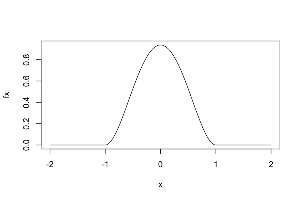
Suppose we want to plot the following function.
\[
f(x) = \begin{cases}
\frac{15}{16} (1 - x^2)^2 & |x| < 1\\
0 & \text{o.w.}
\end{cases}
\]
Take 1:
x = seq(-2, 2, length = 200) ## a vector with the values at which we want to evaluate f
fx = rep(NA, 200) ## pre-allocate a vector in which to store the values of f(x)
for(i in 1:200) {
    if(abs(x[i]) < 1) {
        fx[i] = 15/16 * (1 - x[i]^2)^2
    } else {
        fx[i] = 0
    }
}
plot(fx ~ x, type = 'l')
ifelse: Vectorized conditionals
ifelse syntax:
ifelse(condition, yes, no)
Rules:
ifelse goes element-by-element through condition, yes, and no.
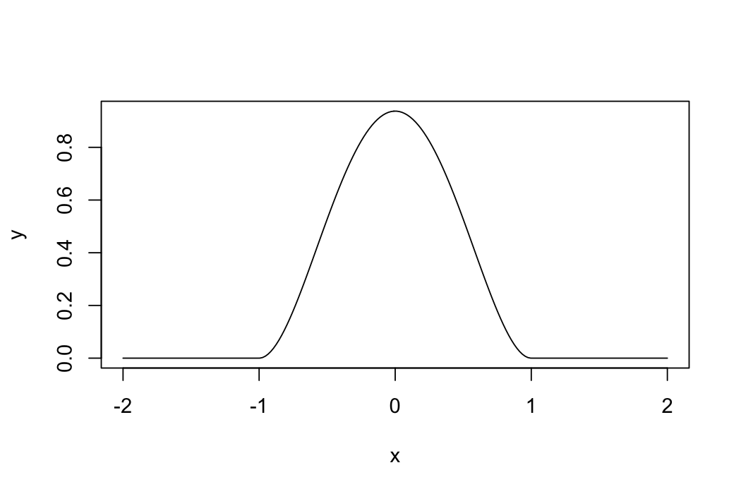
Take 2:
x = seq(-2, 2, length.out = 200)
y = ifelse(abs(x) < 1, 15/16 * (1 - x^2)^2, 0)
plot(y ~ x, type = 'l')
Homework
I'll post a homework on Sunday.
You'll be able to start on it with the material we've covered so far, but it will also cover the text manipulation material we'll go through next week.

