Newton's method
Agenda today
Reading:
- Kenneth Lange, Numerical Analysis for Statisticians, Section 11.2, 13.3
Assignments:
Homework posted on the website, due after spring break
Final project descriptions up on the website, email me by Friday with the project you would like to do and your group.
Maximum likelihood
Problem: We have a family of probability distributions, indexed by a parameter \(\theta\), and we need to choose one to describe the data.
Solution, heuristically:
Assume that our data \(x_1, \ldots, x_n\) are realizations of independent random variables \(X_1, \ldots, X_n\), each coming from the same distribution with parameter \(\theta\).
Find the value of \(\theta\) that makes the data most likely.
Use either the probability density (continuous random variables) or probability mass (discrete random variables) to describe how likely the data is for a given value of the parameter \(\theta\).
Formally:
Let \(f(x; \theta)\) be the probability density function or probability mass function of a random variable with drawn from a distribution with parameter \(\theta\).
With independent data points \(x_1\), \(x_2\), \(x_n\), the likelihood is
\[
L(\theta)=\prod_{i=1}^n f(x_i;\theta)
\]
Recall that the probability density/mass function describes how likely a random variable is to take a given value.
If \(f(x_i; \theta)\) is high, it is very likely that we would see the value \(x_i\) if \(x_i\) really came from a distribution with parameter \(\theta\)
If \(f(x_i; \theta)\) is low, it is unlikely that we would see the value \(x_i\) if \(x_i\) really came from a distribution with parameter \(\theta\)
Therefore: find the value of \(\theta\) that maximizes the likelihood.
In practice, we work with the log likelihood instead of the likelihood:
\[
\ell(\theta) = \sum_{i=1}^n \log f(x_i; \theta)
\]
For example: we have data points \(x_1, \ldots, x_n\), and we want to find the \(N(\theta, 1)\) distribution that fits the data the best.
The likelihood is \[
L(x; \theta) = \prod_{i=1}^n \frac{1}{\sqrt{2\pi}}\exp((x_i - \theta)^2)
\]
and the log likelihood is \[
\ell(x; \theta) = \sum_{i=1}^n\log \left( \frac{1}{\sqrt{2\pi}}\exp((x_i - \theta)^2) \right)
\]
We can use dnorm in R to compute the log likelihood for any \(x\) and \(\theta\) we want:
## create a function that computes the log likelihood
likelihood = function(theta, x) {
    sum(log(dnorm(x, mean = theta, sd = 1)))
}
x = c(5.5, 4, 3.2, 4.7, 4.3, 3.5)
theta_vec = seq(0, 10, length.out = 100)
l_of_theta = sapply(theta_vec, likelihood, x)
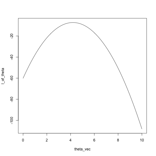
plot(l_of_theta ~ theta_vec, type = 'l')
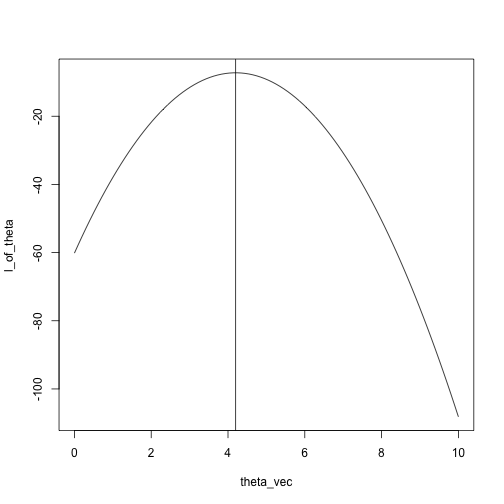
What is the maximum?
plot(l_of_theta ~ theta_vec, type = 'l')
abline(v = mean(x))
Alternately, just search over the grid:
max_idx = which.max(l_of_theta)
theta_vec[max_idx]
## [1] 4.242424
## compare with
mean(x)
## [1] 4.2
Another example: Binomial, five trials, unknown success probability.
likelihood = function(theta, x) {
    sum(log(dbinom(x = x, size = 5, prob = theta)))
}
Compute the likelihoods for many possible values of prob
x = rbinom(n = 100, size = 5, prob = .2)
theta_vec = seq(0, 1, length.out = 100)
log_likelihoods = sapply(theta_vec, likelihood, x)
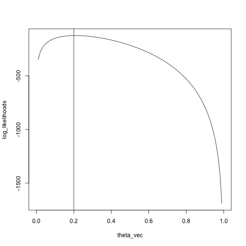
plot(log_likelihoods ~ theta_vec, type = 'l')
abline(v = .2)
We see that the maximum is pretty close to the true value, \(.2\)
max_idx = which.max(log_likelihoods)
theta_vec[max_idx]
## [1] 0.2121212
Newton's method
Iterative method for finding local minimum/maximum of a function.
Also known as Newton-Raphson, after Isaac Newton and Joseph Raphson (Raphson published in 1690, Newton wrote a similar method in 1671 but didn't publish until 1736)
Initial description is for finding zeros of a function
This turns out to be equivalent to an optimization problem/finding maxima of functions, as we need.
Notation
\(\theta\): The parameter(s), either a scalar or a vector.
\(\ell (\theta)\): The log likelihood at \(\theta\).
\(d \ell(\theta)\): The first derivative of the log likelihood at \(\theta\) (if \(\theta\) is a scalar) or the vector of first derivatives of the log likelihood at \(\theta\) (if \(\theta\) is a vector).
\(d^2 \ell(\theta)\): The second derivative of the log likelihood (if \(\theta\) is a scalar) or the matrix of second partial derivatives (if \(\theta\) is a vector.)
What
Our goal: Find the value of \(\theta\) that maximizes \(\ell(\theta)\).
Given that we are at a point \(\theta_n\), one Newton step is given by
\[
\theta_{n+1} = \theta_n - d^2 \ell(\theta_n)^{-1} d \ell(\theta_n)
\]
Newton's method algorithm:
Start at a point \(\theta_0\)
Iterate \(\theta_{n+1} = \theta_n - d^2 \ell(\theta_n)^{-1} d \ell(\theta_n)\) until some stopping criterion is reached.
Usually stop when the derivative is sufficiently close to zero.
Why
Suppose we want to maximze a quadratic:
\[
f(\theta) = a + b \theta + c \theta^2
\]
We can solve for the maximum/minimum analytically by setting the first derivative equal to 0:
\[
d f(\theta) = b + 2 c \theta
\]
If we want \(b + 2c \theta = 0\), we take \(\theta = -\frac{b }{2c}\)
Recast this result as a "step" instead of a single minimization:
We start at \(\theta_0\)
\(\theta_1\) should be \(-\frac{b}{2c}\)
The step is \(\theta_1 - \theta_0\), which is
\[
\theta_1 - \theta_0 = -\frac{b}{2c} - \theta_0 \\
= -\frac{b + 2c \theta_0}{2c} \\
= -\frac{d f(\theta_0)}{d^2 f(\theta_0)}
\]
since \(df(\theta_0) = b + 2c\theta_0\) and \(d^2 f(\theta_0) = 2c\)
Intuition for general, not-necessarily-quadratic functions:
We are not only dealing with quadratic functions, but we can approximate smooth, differentiable functions by quadratic functions.
Taylor approximation of \(\ell(\theta)\) around \(\theta_0\): \[
\ell(\theta) \approx \ell(\theta_0) + d\ell(\theta_0)(\theta - \theta_0) + \frac{1}{2} (\theta - \theta_0)^T d^2 \ell(\theta_0) (\theta - \theta_0)
\]
A Newton step finds an extreme point for the approximation.
Analysis
Newton's method converges very rapidly close to the optimum.
We have the following analytic result:
Let \(\theta^\star\) be the parameter corresponding to a local maximum.
If the second derivative matrix satisfies \[
\|d^2\ell(\phi) - d^2 \ell(\theta)\|\le \lambda \|\phi - \theta\|
\] in some neighborhood of \(\theta^\star\), then the Newton iterates satisfy \[
\|\theta_{n+1} - \theta^\star \|\le 2 \lambda \|d^2 \ell(\theta^\star)^{-1} \| \|\theta_n - \theta^\star\|^2
\]
Note:
The condition on the second derivative matrix means that the curvature doesn't change much in a region around \(\theta^\star\), which you can think of as meaning \(\ell\) is well approximated by a quadratic function.
Larger curvature at the optimum means faster convergence (remember \(-d^2 \ell(\theta)\) is what statisticians call the information).
Potential issues:
\(d \ell\): Does it exist? Can we compute it?
\(d^2\ell\): Does it exist? Can we compute it? Is it invertible?
How do we decide where to start?
Method of moments
Same problem as maximum likelihood: we have a family of probability models, indexed by a scalar or vector \(\theta\), and we need to choose one to describe the data.
Idea:
If \(\theta\) is a \(k\)-dimensional vector (we have \(k\) parameters to estimate), derive expressions for the first \(k\) moments of the data, \(E_\theta(X^r)\), \(r = 1,\ldots, k\)
Compute the first \(k\) moments of the data:
\[
\frac{1}{n} \sum_{i=1}^n x_i^r, \quad r = 1,\ldots, k
\]
\(\hat \theta\) is the value of \(\theta\) such that the empirical moments match the theoretical moments:
\[
E_{\hat \theta}(X^r) = \sum_{i=1}^n x_i^r, \quad r = 1,\ldots, k
\]
Example: moment estimator for normal family
Our family of distributions is \(N(\mu, \sigma^2)\), so that \(\theta = (\mu, \sigma)\).
The first two moments are:
\(E_{\mu, \sigma}(X) = \mu\)
\(E_{\mu, \sigma}(X^2) = \mu^2 + \sigma^2\)
Equate the first theoretical moment to the first data moment tells us that \(\hat \mu\) should satisfy
\[
E_{\hat \mu,\hat \sigma}(X) = \hat \mu = \frac{1}{n} \sum_{i=1}^n x_i
\] and so \(\hat \mu = \frac{1}{n} \sum_{i=1}^n x_i\)
Then equating the second theoretical moments to the second data moment tells us that \(\hat \mu\) and \(\hat \sigma\) should satisfy \[
E_{\mu, \sigma}(X^2) = \mu^2 + \sigma^2 = \frac{1}{n} \sum_{i=1}^n x_i^2
\] Plugging in \(\hat \mu = \sum_{i=1}^n x_i\) and solving gives us \[
E_{\hat \mu, \hat \sigma}(X^2) = \hat \mu^2 + \hat \sigma^2 \\
= (\frac{1}{n} \sum_{i=1}^n x_i)^2 + \hat \sigma^2\\
=\frac{1}{n}\sum_{i=1}^n x_i^2
\] and so \(\hat \sigma^2 = \frac{1}{n}\sum_{i=1}^n x_i^2 - (\frac{1}{n}\sum_{i=1}^n x_i)^2\).
If you do a little more algebra, you can see that this is a standard estimate of the variance.
Example: moment estimator for mixture models
Mixture model
\(x_1, \ldots, x_n\) come from a distribution with cumulative distribution function \(\theta G + (1 - \theta)H\), where \(G\) and \(H\) are two fixed, distributions (for example, two normal distributions with known means and variances, or two Poisson distributions with different means).
Let \(\xi\) denote the mean of \(G\) and \(\eta\) denote the mean of \(H\).
We want to estimate the mixing parameter \(\theta\).
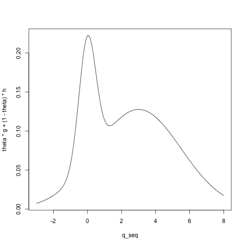
For example, we can visualize the density for a mixture of a \(N(0, .5)\) and a \(N(3, 2.5)\) distribution with mixing parameter \(\theta = .2\):
mean_G = 0
mean_H = 3
sd_G = .5
sd_H = 2.5
q_seq = seq(-3, 8, length.out = 1000)
g = dnorm(q_seq, mean = mean_G, sd = sd_G)
h = dnorm(q_seq, mean = mean_H, sd = sd_H)
theta = .2
plot(theta * g + (1 - theta) * h ~ q_seq, type = 'l')
We have one parameter, so we compute the first theoretical moment: \[
E_\theta(X) = \theta \xi + (1 - \theta) \eta
\]
Then we equate that moment to the first data moment to get our estimate: \[
\hat \theta \xi + (1 - \hat \theta) \eta = \frac{1}{n} \sum_{i=1}^n x_i\\
\hat \theta = \frac{\frac{1}{n} \sum_{i=1}^n x_i - \eta}{\xi - \eta}
\]
There isn't anything particularly important about the first \(k\) moments, can match other aspects of the data
We are thinking of these as starting values for maximum likelihood estimation, but they are usually reasonable estimators in their own right.
The idea of matching data statistics to expected values of statistics will come up again in approximate Bayesian computation.


