Stat 470/670 Lecture 3

Julia Fukuyama

Today: Comparing many univariate distributions

Tidy data/reshaping

Measures of center and spread

Boxplots

Computational Interlude: Tidy Data

Reading: http://r4ds.had.co.nz/tidy-data.html

Tidy data means:

Every column is a variable.

Every row is an observation.

Every element is a value.

library(tidyverse)
table1

## # A tibble: 6 × 4
##   country      year  cases population
##   <chr>       <int>  <int>      <int>
## 1 Afghanistan  1999    745   19987071
## 2 Afghanistan  2000   2666   20595360
## 3 Brazil       1999  37737  172006362
## 4 Brazil       2000  80488  174504898
## 5 China        1999 212258 1272915272
## 6 China        2000 213766 1280428583

table2

## # A tibble: 12 × 4
##    country      year type            count
##    <chr>       <int> <chr>           <int>
##  1 Afghanistan  1999 cases             745
##  2 Afghanistan  1999 population   19987071
##  3 Afghanistan  2000 cases            2666
##  4 Afghanistan  2000 population   20595360
##  5 Brazil       1999 cases           37737
##  6 Brazil       1999 population  172006362
##  7 Brazil       2000 cases           80488
##  8 Brazil       2000 population  174504898
##  9 China        1999 cases          212258
## 10 China        1999 population 1272915272
## 11 China        2000 cases          213766
## 12 China        2000 population 1280428583

table3

## # A tibble: 6 × 3
##   country      year rate             
## * <chr>       <int> <chr>            
## 1 Afghanistan  1999 745/19987071     
## 2 Afghanistan  2000 2666/20595360    
## 3 Brazil       1999 37737/172006362  
## 4 Brazil       2000 80488/174504898  
## 5 China        1999 212258/1272915272
## 6 China        2000 213766/1280428583

table4a

## # A tibble: 3 × 3
##   country     `1999` `2000`
## * <chr>        <int>  <int>
## 1 Afghanistan    745   2666
## 2 Brazil       37737  80488
## 3 China       212258 213766

table4b

## # A tibble: 3 × 3
##   country         `1999`     `2000`
## * <chr>            <int>      <int>
## 1 Afghanistan   19987071   20595360
## 2 Brazil       172006362  174504898
## 3 China       1272915272 1280428583

Pipes

The magrittr library offers the “pipe” operation, %>%.

In words: “Pipe the output of the last function as input to the next function”.

Suppose f1 and f2 are functions. These are equivalent:

f2(f1(x))

f1(x) %>% f2()

The output of f1(x) is used as the first argument to f2.

For example:

head(seq(.5, 11, by = 1))

## [1] 0.5 1.5 2.5 3.5 4.5 5.5

seq(.5, 11, by = 1) %>% head()

## [1] 0.5 1.5 2.5 3.5 4.5 5.5

Pivot longer

Problem: some of the column names are not names of variables, but values of a variable

To solve this problem, we need to pivot longer. To describe that operation, we need three parameters:

The set of columns whose names are values, not variables.

The name of the variable to move the column names to.

The name of the variable to move the column values to.

table4a %>%
    pivot_longer(c(`1999`, `2000`), names_to = "year", values_to = "cases") %>%
    head(n = 3)

## # A tibble: 3 × 3
##   country     year  cases
##   <chr>       <chr> <int>
## 1 Afghanistan 1999    745
## 2 Afghanistan 2000   2666
## 3 Brazil      1999  37737

head(pivot_longer(table4a, c(`1999`, `2000`), names_to = "year", values_to = "cases"), n = 3)

## # A tibble: 3 × 3
##   country     year  cases
##   <chr>       <chr> <int>
## 1 Afghanistan 1999    745
## 2 Afghanistan 2000   2666
## 3 Brazil      1999  37737

Pivot wider

Problem: an observation is scattered across multiple rows.

To solve this problem, we need to pivot wider. To describe that operation, we need two parameters:

The column to take variable names from.

The column to take values from.

table2

## # A tibble: 12 × 4
##    country      year type            count
##    <chr>       <int> <chr>           <int>
##  1 Afghanistan  1999 cases             745
##  2 Afghanistan  1999 population   19987071
##  3 Afghanistan  2000 cases            2666
##  4 Afghanistan  2000 population   20595360
##  5 Brazil       1999 cases           37737
##  6 Brazil       1999 population  172006362
##  7 Brazil       2000 cases           80488
##  8 Brazil       2000 population  174504898
##  9 China        1999 cases          212258
## 10 China        1999 population 1272915272
## 11 China        2000 cases          213766
## 12 China        2000 population 1280428583

table2 %>%
    pivot_wider(names_from = type, values_from = count)

## # A tibble: 6 × 4
##   country      year  cases population
##   <chr>       <int>  <int>      <int>
## 1 Afghanistan  1999    745   19987071
## 2 Afghanistan  2000   2666   20595360
## 3 Brazil       1999  37737  172006362
## 4 Brazil       2000  80488  174504898
## 5 China        1999 212258 1272915272
## 6 China        2000 213766 1280428583

Mean and Standard Deviation

Our observations are \(x_1, \ldots, x_n\)

Sample mean: \[ \text{mean}(x_1,\ldots, x_n) = \frac{1}{n} \sum_{i=1}^n x_i \]

Standard deviation: \[ \text{sd}(x_1, \ldots, x_n) = \sqrt{\frac{1}{n-1} \sum_{i=1}^n (x_i - \text{mean}(x_1,\ldots, x_n))^2} \]

Some drawbacks

Mean and standard deviation are good if you have normal data (how would we check this?)

What if our data are not normal?

What if they are highly skewed? (e.g. income data, house price data)

What if some fraction of the values are corrupted? (e.g. someone coded missing values as 999)

Breakdown point

Let \(x_1, \ldots, x_n\) be a sample of size \(n\).

Suppose we add \(y_1, \ldots, y_m\) “bad” samples to \(x_1, \ldots, x_n\), to get a corrupted dataset \(x_1, \ldots, x_n, y_1, \ldots, y_m\).

We are interested in the value of a function \(f\) (e.g. the mean, \(f((x_1, \ldots, x_n)) = \sum_{i=1}^n x_i / n\)).

The breakdown point of the function \(f\) is \(\frac{m}{m+n}\) for the smallest value of \(m\) required to make \(f((x_1, \ldots, x_n, y_1, \ldots, y_m))\) arbitrarily different from \(f(x_1, \ldots, x_n)\).

Functions with high breakdown points are robust, insensitive to corruption and outliers.

Robust measures of center

Suppose our sorted observations are \(x_{(1)}, \ldots, x_{(n)}\)

Median: If \(n\) is odd, \[\text{med}(x_{(1)}, \ldots, x_{(n)}) = x_{((n+1)/2)}\] If \(n\) is even, we can use \[\text{med}(x_{(1)}, \ldots, x_{(n)}) = \frac{1}{2}x_{(n/2)} + \frac{1}{2}x_{(n/2 + 1)}\]

\(\alpha\)-trimmed mean: Drop the \(\alpha n\) lowest and highest observations, take the mean of the remainder.

\(\alpha\)-winsorized mean: Assuming \(\alpha n\) is a whole number: Replace the \(\alpha n\) lowest and highest observations with \(x_{(\alpha n + 1)}\) and \(x_{((1 - \alpha) n - 1)}\), respectively. Take the mean of the modified values.

What are their breakdown points?

Robust measures of spread

Median absolute deviation: \[ \text{mad}(x_1, \ldots, x_n) = \text{med} (|x_1 - \text{med}(x_1, \ldots, x_n)|, \ldots, |x_n - \text{med}(x_1, \ldots, x_n)|) \]

Interquartile range: If \(.25n\) and \(.75n\) are whole numbers, then \[ \text{iqr}(x_1,\ldots, x_n) = x_{(.75n)} - x_{(.25n)} \]

What are their breakdown points? Can you think of other robust measures of spread?

Tradeoffs

Why would we want to use a less robust estimator?

Tradeoff between efficiency and robustness

Robust version might not estimate what you want, or could be biased for the quantity you want

Computational Interlude: Aggregation

dplyr makes it easy to compute data summaries.

The summarise function will compute a summary statistic of one of the variables in the data table.

If you call group_by before summarise, summarise will compute the statistic for each value of the grouped variable.

library(dplyr)
## for the data
library(lattice)
singer %>% summarise(median(height))

##   median(height)
## 1             67

summarise(singer, median(height))

##   median(height)
## 1             67

singer %>% group_by(voice.part) %>% summarise(median(height))

## # A tibble: 8 × 2
##   voice.part `median(height)`
##   <fct>                 <dbl>
## 1 Bass 2                   72
## 2 Bass 1                   71
## 3 Tenor 2                  69
## 4 Tenor 1                  68
## 5 Alto 2                   66
## 6 Alto 1                   65
## 7 Soprano 2                64
## 8 Soprano 1                65

summarise(group_by(singer, voice.part), median(height))

## # A tibble: 8 × 2
##   voice.part `median(height)`
##   <fct>                 <dbl>
## 1 Bass 2                   72
## 2 Bass 1                   71
## 3 Tenor 2                  69
## 4 Tenor 1                  68
## 5 Alto 2                   66
## 6 Alto 1                   65
## 7 Soprano 2                64
## 8 Soprano 1                65

Boxplots

Goal:

More parsimonious representation of the distribution.

Why do we want this? Shouldn’t we always try to keep all the data?

Boxplot Statistics

Suppose our data is \(x_1, \ldots, x_n\). We compute five statistics of the data:

\(q_x(.5)\), the median.

\(q_x(.25)\), the .25 quantile of \(x_1, \ldots, x_n\) aka the lower quartile

\(q_x(.75)\), the .75 quantile of \(x_1, \ldots, x_n\) aka the upper quartile

Upper adjacent value (UAV), lower adjacent value (LAV)

\[r =q_x(.75) - q_x(.25)\]

\[\text{UAV} = \text{max} \{ x_i : x_i \le q_{.75} + 1.5r \}\]

\[\text{LAV} = \text{min} \{ x_i : x_i \ge q_{.25} - 1.5r \}\]

Note that these are all robust statistics

Reading a Boxplot

Bar in the middle represents the median.

Edges of box represent \(q_x(.25)\) and \(q_x(.75)\).

Whiskers represent the UAV and LAV.

Any values outside of the range \([\text{LAV}, \text{UAV}]\) are referred to as outside values and are plotted individually.

Boxplot Demonstration

We can make a boxplot of just one variable, but only by hacking the syntax a bit (because the primary purpose of a boxplot is to compare multiple distributions).

library(ggplot2)
## lattice is for the singer data
library(lattice)
ggplot(singer, aes(x = "Height", y = height)) +
    geom_boxplot()

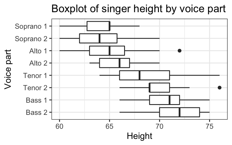
More useful is to compare boxplots of the different voice parts.

ggplot(singer, aes(x = voice.part, y = height)) +
    geom_boxplot() +
    coord_flip() +
    ggtitle("Boxplot of singer height by voice part") +
    ylab("Height") + xlab("Voice part")

Training our intuition

How should we think about upper and lower adjacent values?

We can compute them for normally distributed data:

(iqr = qnorm(.75) - qnorm(.25))

## [1] 1.34898

(uav = qnorm(.75) + 1.5 * iqr)

## [1] 2.697959

(lav = qnorm(.25) - 1.5 * iqr)

## [1] -2.697959

We can also ask what the probability any single point is an outside point for normally distributed data:

(prob_outside = pnorm(uav, lower.tail = FALSE) + pnorm(lav, lower.tail = TRUE))

## [1] 0.006976603

Or the probability of at least one outside point if we have 30 observations:

n = 30
1 - (1 - prob_outside)^n

## [1] 0.1894414

Or the probability of at least one outside point if we have 3000 observations

n = 3000
1 - (1 - prob_outside)^n

## [1] 1

Note: These are approximations, we’re computing the probability that we get a point outside of the range of the large-sample upper- and lower-adjacent values, which is slightly different than the probability of an outside point. If you want a good math problem you might have fun working out the true probabilities, but otherwise the approximation is good enough for training our intuition.

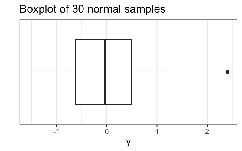
What do boxplots look like with normal data?

We saw that if we have 30 observations, we don’t expect many outside values from normally distributed data:

set.seed(0)
df = data.frame(y = rnorm(30), x = "")
ggplot(df) +
    geom_boxplot(aes(x = x, y = y)) +
    coord_flip() + xlab("") + ggtitle("Boxplot of 30 normal samples")

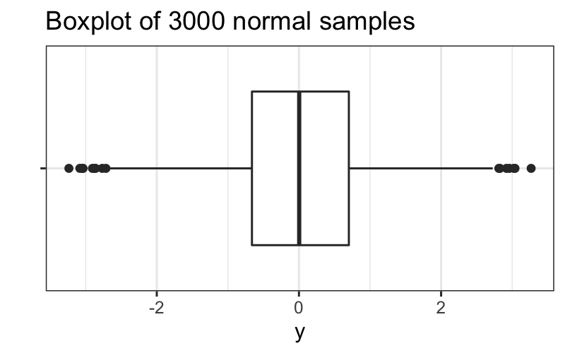
But if we have 3000 observations, we expect to get a lot:

set.seed(0)
df = data.frame(y = rnorm(3000), x = "")
ggplot(df) +
    geom_boxplot(aes(x = x, y = y)) +
    coord_flip() + xlab("") + ggtitle("Boxplot of 3000 normal samples")