Stat 470/670 Lecture 24: Scree plots and choosing the number of dimensions

Julia Fukuyama

Today

Scree plot and how we interpret it
What does the scree plot look like when the data matrix is just noise
How do we choose a good number of dimensions for PCA

Scree plots

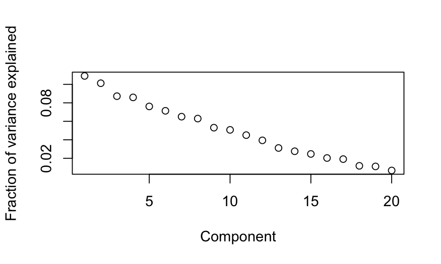
In a scree plot, we plot the eigenvalues in decreasing order.

It is used to help us choose the number of “important” principal components.

Scree plot: Advice

Look for an elbow (the plot is supposed to look like a scree).

Take as many components as necessary to get to at least some pre-determined fraction of variance explained.

Compare eigenvalues to a null distribution.

Three simulated examples

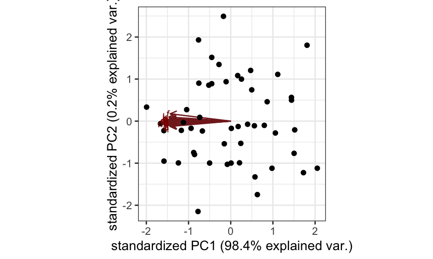
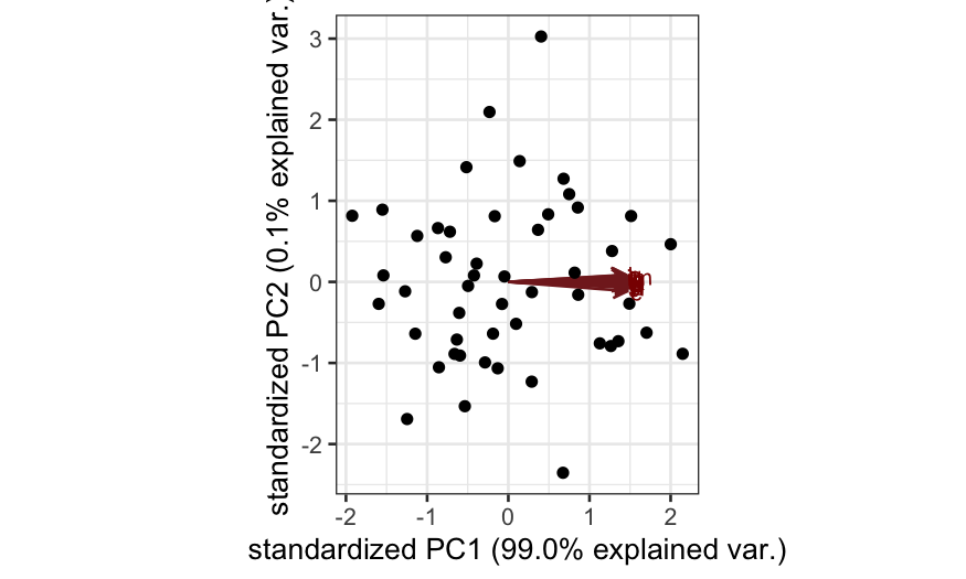
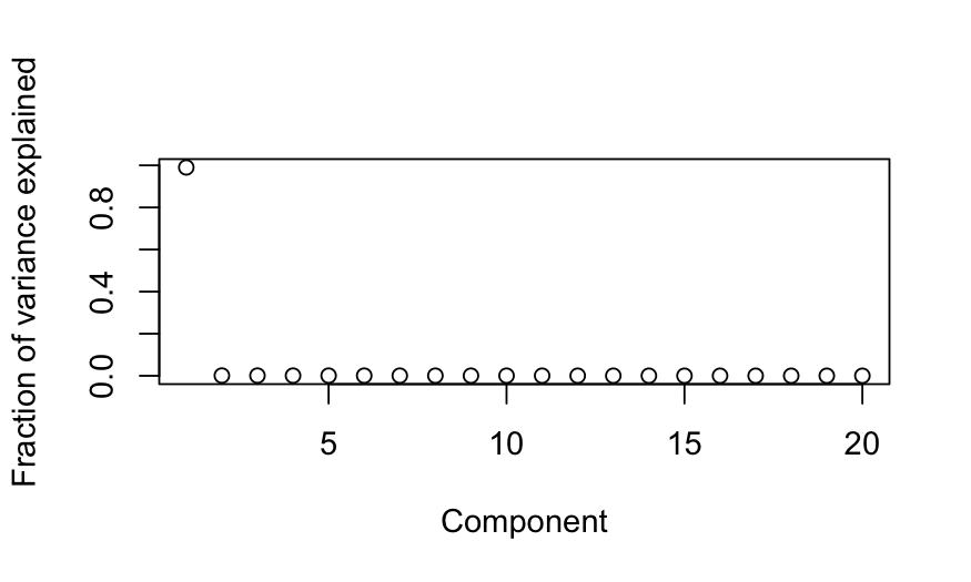
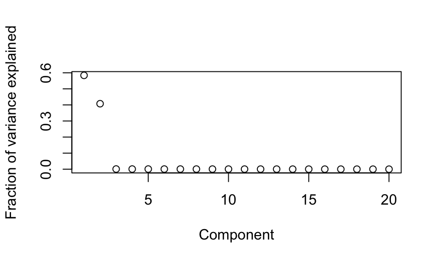
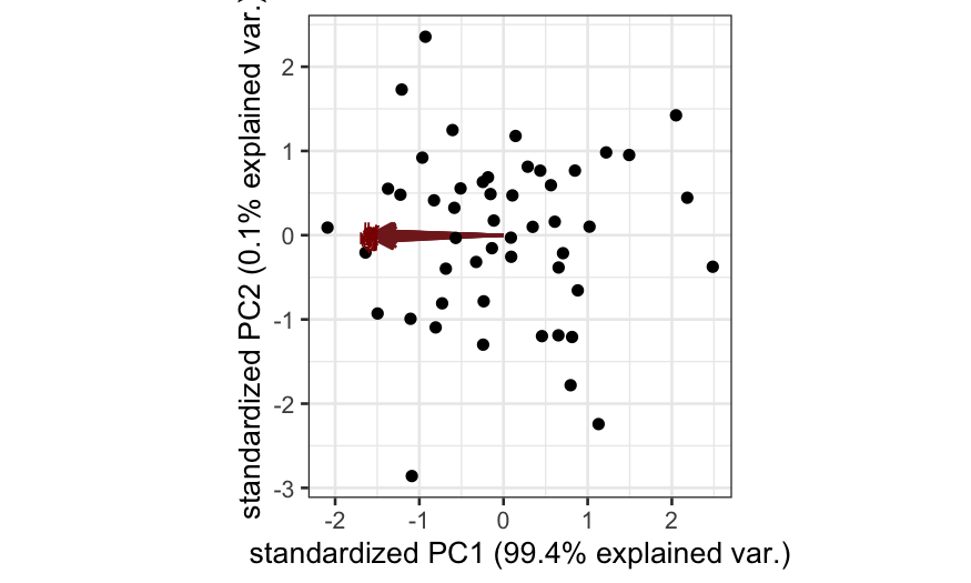
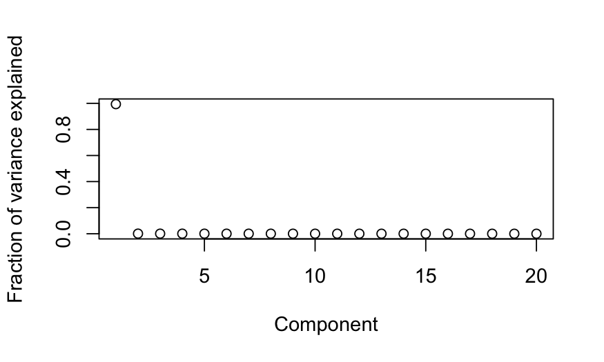
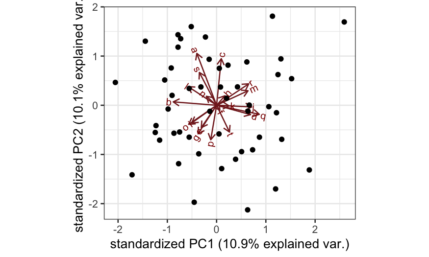
Simulation A: All of the variables are highly correlated with each other. Interpretation: all of the variables are measuring the same underlying quantity.

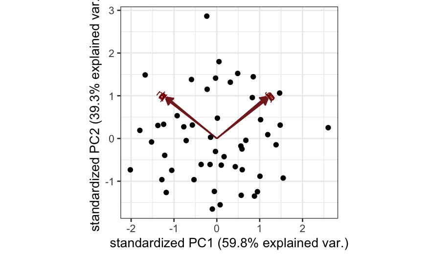
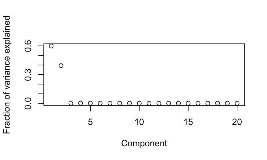
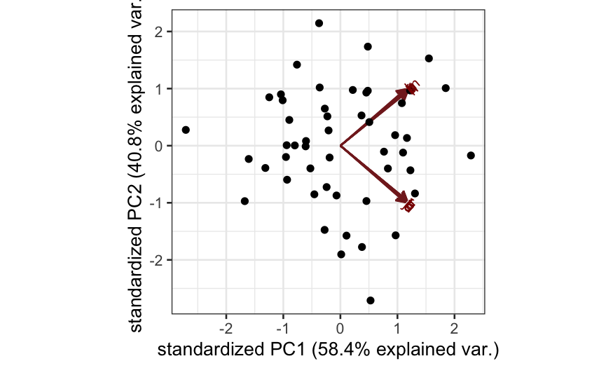
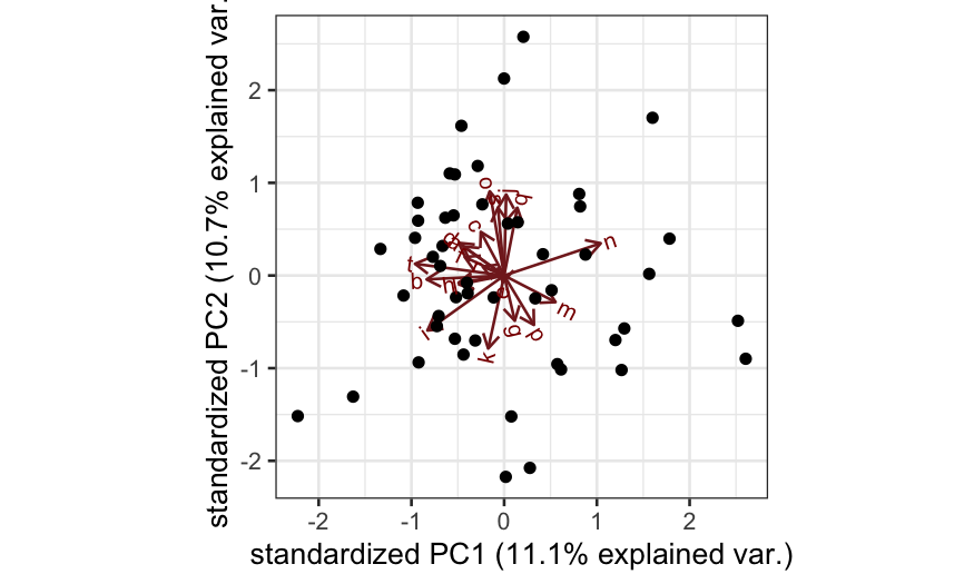
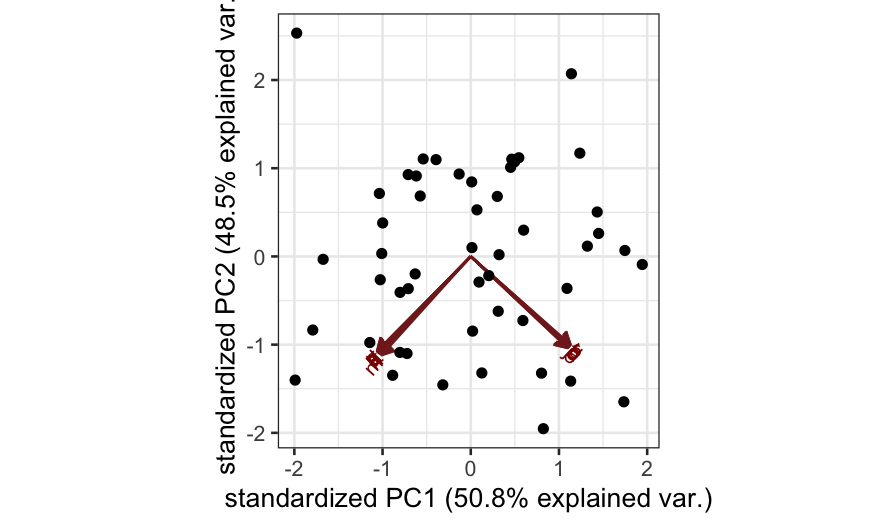
Simulation B: There are two blocks of variables, with high correlations within each block. Interpretation: there are two independent underlying factors, and each of the variables measures one of them.

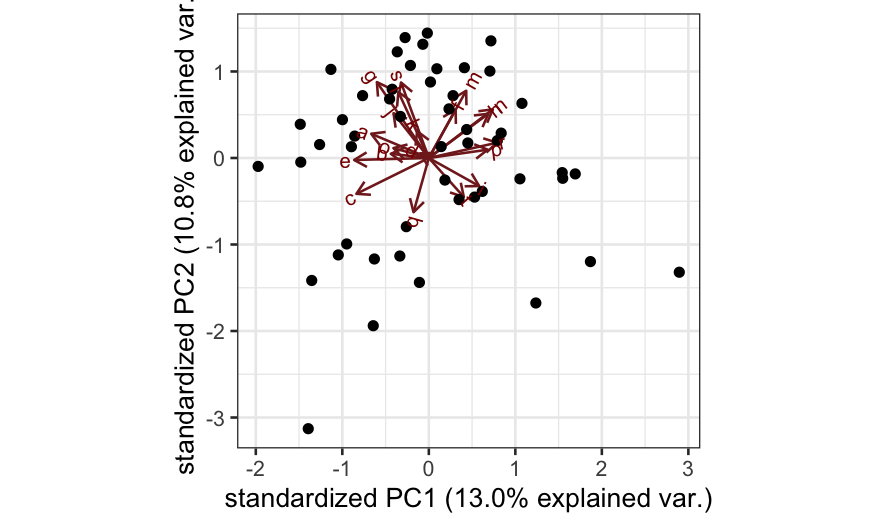
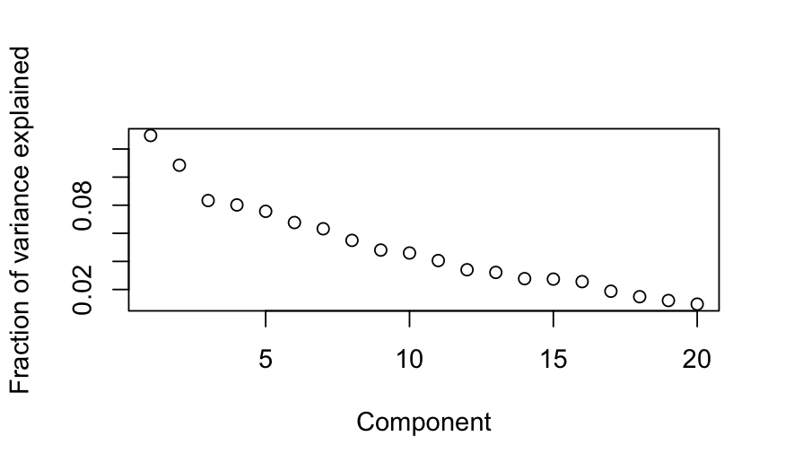
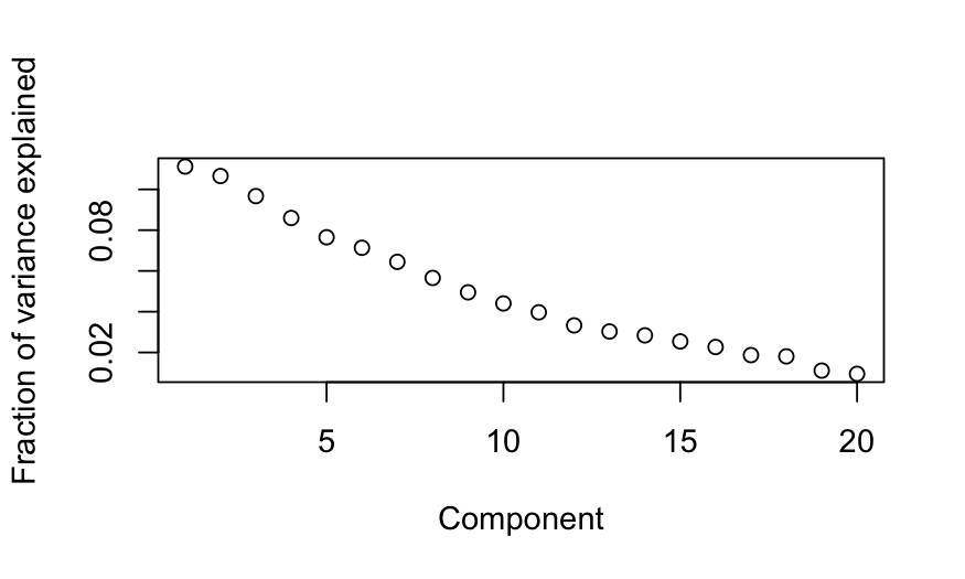
Simulation C: All of the variables are independent. Interpretation: there is no lower-dimensional structure to uncover with PCA.

Simulation A

n = 50; p = 20
cov.mat = matrix(.99, nrow = p, ncol = p)
diag(cov.mat) = 1
X = rmvnorm(n = n, sigma = cov.mat)
colnames(X) = letters[1:p]
out_prcomp = prcomp(X, center = TRUE, scale. = FALSE)
ggbiplot(out_prcomp)

plot(out_prcomp$sdev^2 / sum(out_prcomp$sdev^2),
     ylab = "Fraction of variance explained", xlab = "Component")

Simulation B

cov.mat = matrix(0, nrow = p, ncol = p)
cov.mat[1:(p/2), 1:(p/2)] = cov.mat[(p/2 + 1):p, (p/2 + 1):p] = .99
diag(cov.mat) = 1
X = rmvnorm(n = n, sigma = cov.mat)
colnames(X) = letters[1:p]
out_prcomp = prcomp(X, center = TRUE, scale. = TRUE)
ggbiplot(out_prcomp)

plot(out_prcomp$sdev^2 / sum(out_prcomp$sdev^2),
     ylab = "Fraction of variance explained", xlab = "Component")

Simulation C

X = matrix(rnorm(n * p), nrow = n)
colnames(X) = letters[1:p]
out_prcomp = prcomp(X, center = TRUE, scale. = TRUE)
ggbiplot(out_prcomp)

plot(out_prcomp$sdev^2 / sum(out_prcomp$sdev^2),
     ylab = "Fraction of variance explained", xlab = "Component")

Comparing to a null distribution

Assuming the elements of the data matrix are iid Gaussians or the sample covariance matrix has a Wishart distribution, the limiting distributions of the eigenvalues have been worked out.

The distribution of the largest eigenvalue follows the Tracy-Widom law. (Also: an article in Quanta)

The empirical distribution of the eigenvalues will converge to the Marcenko-Pastur distribution.

These limits are a bit different than what you see in your other statistical theory courses, they are based on taking both the number of samples and the number of variables to infinity in a fixed ratio.

The package RMTstat contains the relevant distributions, we will use pWishartMax for the distribution of the maximum eigenvalue of a Wishart matrix.

Simulation A

n = 50; p = 20
cov.mat = matrix(.99, nrow = p, ncol = p)
diag(cov.mat) = 1
X = rmvnorm(n = n, sigma = cov.mat)
colnames(X) = letters[1:p]
out_prcomp = prcomp(X, center = TRUE, scale. = FALSE)
ggbiplot(out_prcomp)

plot(out_prcomp$sdev^2 / sum(out_prcomp$sdev^2),
     ylab = "Fraction of variance explained", xlab = "Component")

pWishartMax(out_prcomp$sdev[1]^2, ndf = n, pdim = p, lower.tail = FALSE)

## [1] 0

Simulation B

cov.mat = matrix(0, nrow = p, ncol = p)
cov.mat[1:(p/2), 1:(p/2)] = cov.mat[(p/2 + 1):p, (p/2 + 1):p] = .99
diag(cov.mat) = 1
X = rmvnorm(n = n, sigma = cov.mat)
colnames(X) = letters[1:p]
out_prcomp = prcomp(X, center = TRUE, scale. = TRUE)
ggbiplot(out_prcomp)

plot(out_prcomp$sdev^2 / sum(out_prcomp$sdev^2),
     ylab = "Fraction of variance explained", xlab = "Component")

pWishartMax(out_prcomp$sdev[1]^2, ndf = n, pdim = p, lower.tail = FALSE)

## [1] 0

Simulation C

X = matrix(rnorm(n * p), nrow = n)
colnames(X) = letters[1:p]
out_prcomp = prcomp(X, center = TRUE, scale. = TRUE)
ggbiplot(out_prcomp)

plot(out_prcomp$sdev^2 / sum(out_prcomp$sdev^2),
     ylab = "Fraction of variance explained", xlab = "Component")

pWishartMax(out_prcomp$sdev[1]^2, ndf = n, pdim = p, lower.tail = FALSE)

## [1] 0.8334145

Comparing to a null distirbution: Parallel analysis

Suppose you don’t want to assume that the elements of the data matrix are iid Gaussian, or you don’t have a large number of samples/variables. You can use parallel analysis.

Procedure:

Permute each of the columns of the matrix.

Compute the eigenvalues for the permuted data matrix.

Repeat many times.

Compare observed eigenvalues to the eigenvalues computed from the permuted data matrix.

This procedure gives the distribution of the eigenvalues assuming that the variables are uncorrelated and can tell you whether the eigenvalues you observed are bigger than you would expect if all the variables were uncorrelated.

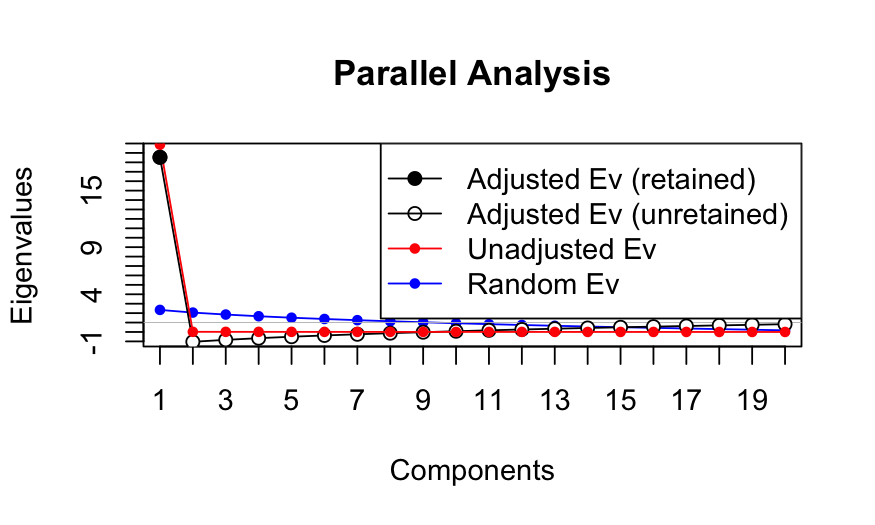
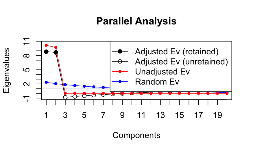
Note: the plots will have “adjusted” eigenvalues, for a description of these see https://alexisdinno.com/Software/files/PA_for_PCA_vs_FA.pdf

Simulation A

n = 50; p = 20
cov.mat = matrix(.99, nrow = p, ncol = p)
diag(cov.mat) = 1
X = rmvnorm(n = n, sigma = cov.mat)
colnames(X) = letters[1:p]
out_prcomp = prcomp(X, center = TRUE, scale. = FALSE)
ggbiplot(out_prcomp)

plot(out_prcomp$sdev^2 / sum(out_prcomp$sdev^2),
     ylab = "Fraction of variance explained", xlab = "Component")

paran(X, graph = TRUE)

## 
## Using eigendecomposition of correlation matrix.
## Computing: 10%  20%  30%  40%  50%  60%  70%  80%  90%  100%
## 
## 
## Results of Horn's Parallel Analysis for component retention
## 600 iterations, using the mean estimate
## 
## -------------------------------------------------- 
## Component   Adjusted    Unadjusted    Estimated 
##             Eigenvalue  Eigenvalue    Bias 
## -------------------------------------------------- 
## 1          18.536246   19.877931      1.341684
## -------------------------------------------------- 
## 
## Adjusted eigenvalues > 1 indicate dimensions to retain.
## (1 components retained)

Simulation B

cov.mat = matrix(0, nrow = p, ncol = p)
cov.mat[1:(p/2), 1:(p/2)] = cov.mat[(p/2 + 1):p, (p/2 + 1):p] = .99
diag(cov.mat) = 1
X = rmvnorm(n = n, sigma = cov.mat)
colnames(X) = letters[1:p]
out_prcomp = prcomp(X, center = TRUE, scale. = TRUE)
ggbiplot(out_prcomp)

plot(out_prcomp$sdev^2 / sum(out_prcomp$sdev^2),
     ylab = "Fraction of variance explained", xlab = "Component")

paran(X, graph = TRUE)

## 
## Using eigendecomposition of correlation matrix.
## Computing: 10%  20%  30%  40%  50%  60%  70%  80%  90%  100%
## 
## 
## Results of Horn's Parallel Analysis for component retention
## 600 iterations, using the mean estimate
## 
## -------------------------------------------------- 
## Component   Adjusted    Unadjusted    Estimated 
##             Eigenvalue  Eigenvalue    Bias 
## -------------------------------------------------- 
## 1           8.801628   10.153689      1.352060
## 2           8.654407   9.707843      1.053435
## -------------------------------------------------- 
## 
## Adjusted eigenvalues > 1 indicate dimensions to retain.
## (2 components retained)

Simulation C

X = matrix(rnorm(n * p), nrow = n)
colnames(X) = letters[1:p]
out_prcomp = prcomp(X, center = TRUE, scale. = TRUE)
ggbiplot(out_prcomp)

plot(out_prcomp$sdev^2 / sum(out_prcomp$sdev^2),
     ylab = "Fraction of variance explained", xlab = "Component")

paran(X, graph = TRUE)

## 
## Using eigendecomposition of correlation matrix.
## Computing: 10%  20%  30%  40%  50%  60%  70%  80%  90%  100%
## 
## 
## Results of Horn's Parallel Analysis for component retention
## 600 iterations, using the mean estimate
## 
## -------------------------------------------------- 
## Component   Adjusted    Unadjusted    Estimated 
##             Eigenvalue  Eigenvalue    Bias 
## -------------------------------------------------- 
## 1           0.842456    2.181949      1.339493

## Error in if (AdjEv[x] >= 0) {: argument is of length zero

Example: Congressional voting data

A dataset containing information about votes taken by Senators in the 1999 session.

Information split across three different csvs, one giving the votes, one giving information about the members, and one giving information about the bills being voted on.

# read in the three data sets
vote_descriptions = read.csv("../../datasets/congress_1999/bills.csv")
members = read.csv("../../datasets/congress_1999/members.csv")
votes = read.csv("../../datasets/congress_1999/votes.csv")
## match the column names of votes and the vote_id column in vote_descriptions
vote_descriptions = vote_descriptions %>%
    mutate(vote_id = str_replace(vote_id, "-", "."))

## match names and orders for members and votes
joined = join(members, votes, by = "id")
votes = joined[,(-1:-6)]
members = joined[,1:6]

## Look at the vote_descriptions data frame
table(vote_descriptions$category)

## 
##  amendment    cloture conviction nomination    passage procedural     treaty 
##        103         36          2         10         61        161          1

We would like to perform PCA, so we need te recode the votes from Yea/Nay to a number.

## Decide how to recode the variables
recode_votes = function(vote) {
    if(is.na(vote)) {
        return(0)
    } else if(vote == "Yea") {
        return(1)
    } else if(vote == "Nay") {
        return(-1)
    } else {
        return(0)
    }
}
votes_numeric = apply(votes, 1:2, recode_votes)
## These votes are going to cause problems for parallel analysis, so we remove them
votes_to_remove = which(apply(votes_numeric, 2, sd) == 0)
votes_numeric = votes_numeric[,-votes_to_remove]
vote_descriptions = vote_descriptions[-votes_to_remove,]

## PCA
out_prcomp = prcomp(votes_numeric)

## scree plot
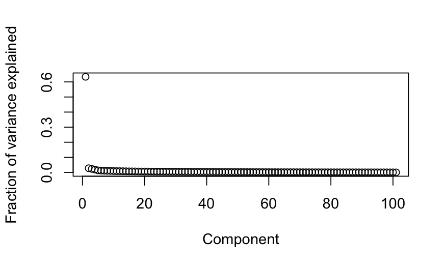
plot(out_prcomp$sdev^2 / sum(out_prcomp$sdev^2),
     xlab = "Component", ylab = "Fraction of variance explained")

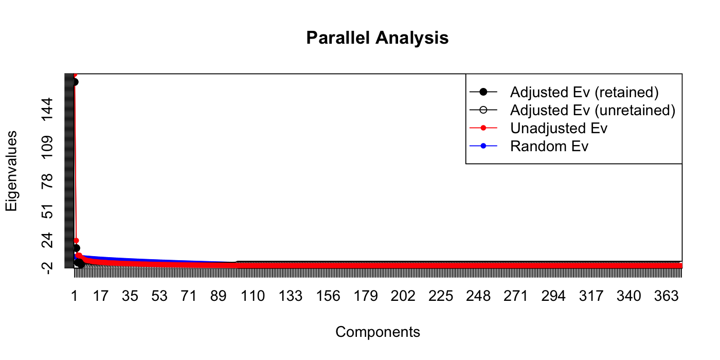
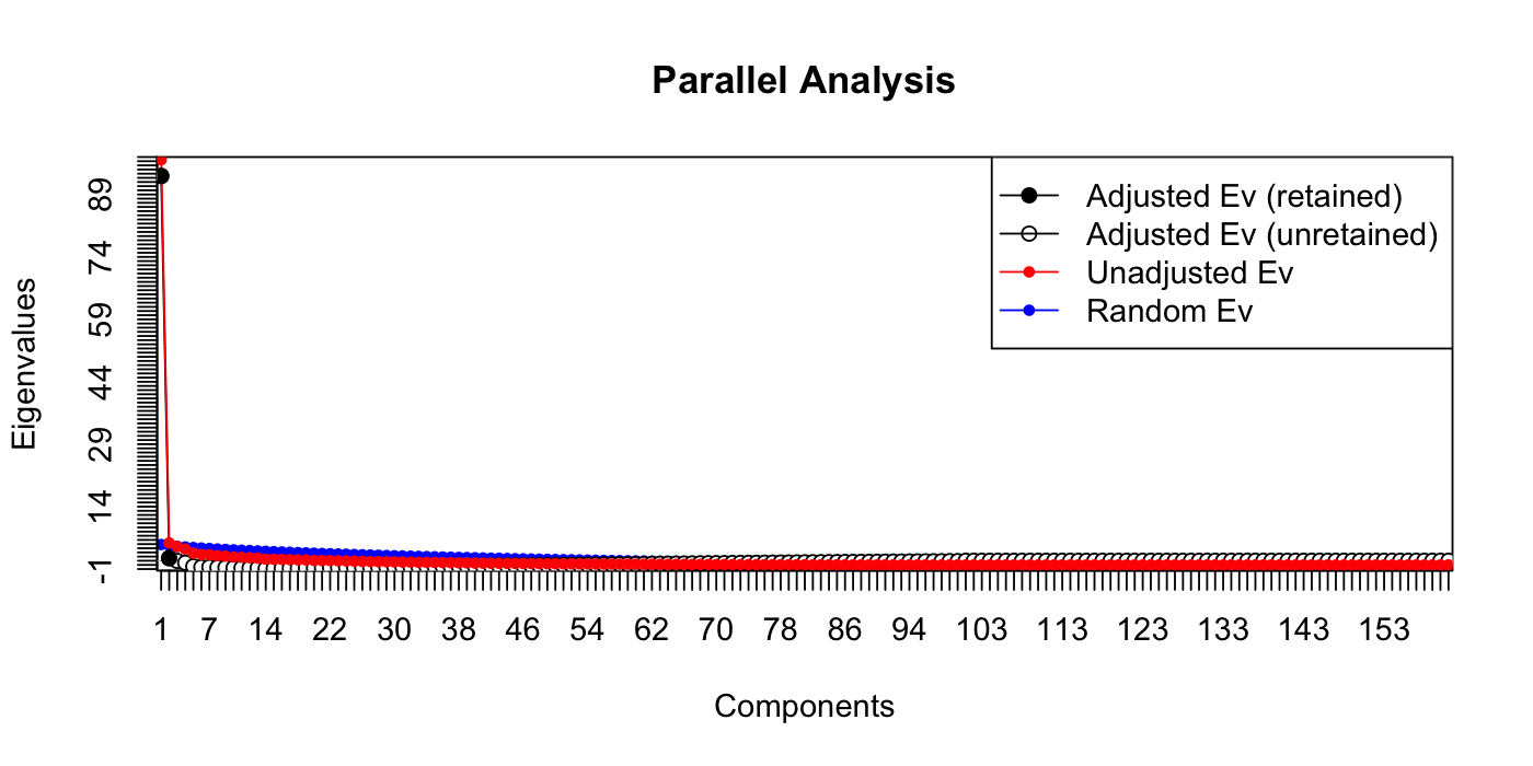
paran(votes_numeric, graph = TRUE, iterations = 100)

## 
## Using eigendecomposition of correlation matrix.
## Computing: 10%  20%  30%  40%  50%  60%  70%  80%  90%  100%
## 
## 
## Results of Horn's Parallel Analysis for component retention
## 100 iterations, using the mean estimate
## 
## -------------------------------------------------- 
## Component   Adjusted    Unadjusted    Estimated 
##             Eigenvalue  Eigenvalue    Bias 
## -------------------------------------------------- 
## 1         169.50319  176.781706      7.278510
## 2          16.274826   23.231897      6.957071
## 3           2.875923   9.615791      6.739868
## 4           3.023778   9.557597      6.533818
## 5           1.109663    7.472130      6.362466
## -------------------------------------------------- 
## 
## Adjusted eigenvalues > 1 indicate dimensions to retain.
## (5 components retained)

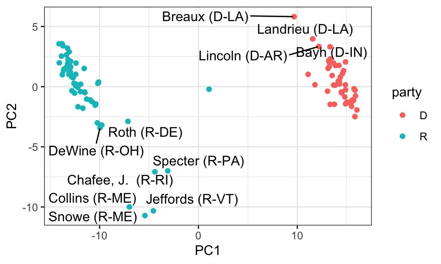
## let's look at who the senators are
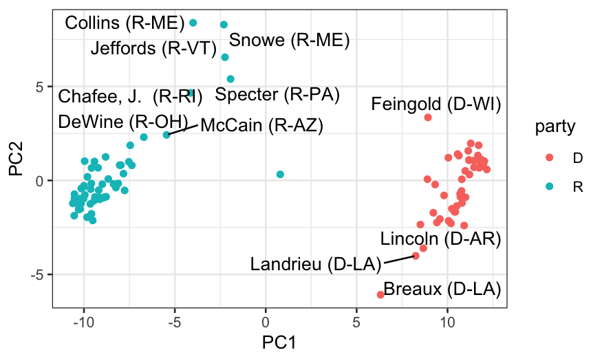
members_and_scores = data.frame(members, out_prcomp$x)
ggplot(members_and_scores, aes(x = PC1, y = PC2)) +
    geom_point(aes(color = party)) +
    geom_text_repel(aes(label = display_name))

Looking at just the “passage” votes

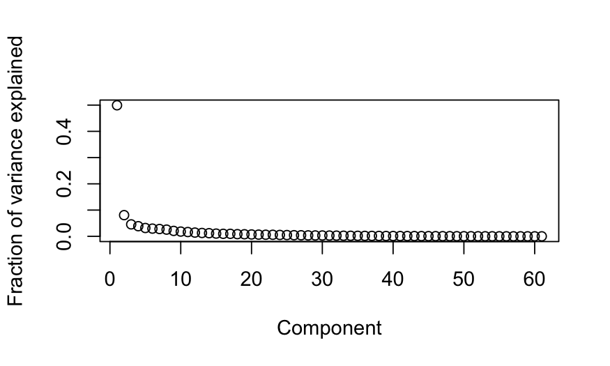
out_prcomp_passage = prcomp(votes_numeric[,vote_descriptions$category == "passage"])
plot(out_prcomp_passage$sdev^2 / sum(out_prcomp_passage$sdev^2),
     ylab = "Fraction of variance explained", xlab = "Component")

out_prcomp_passage$sdev[1]^2 / sum(out_prcomp_passage$sdev^2)

## [1] 0.499316

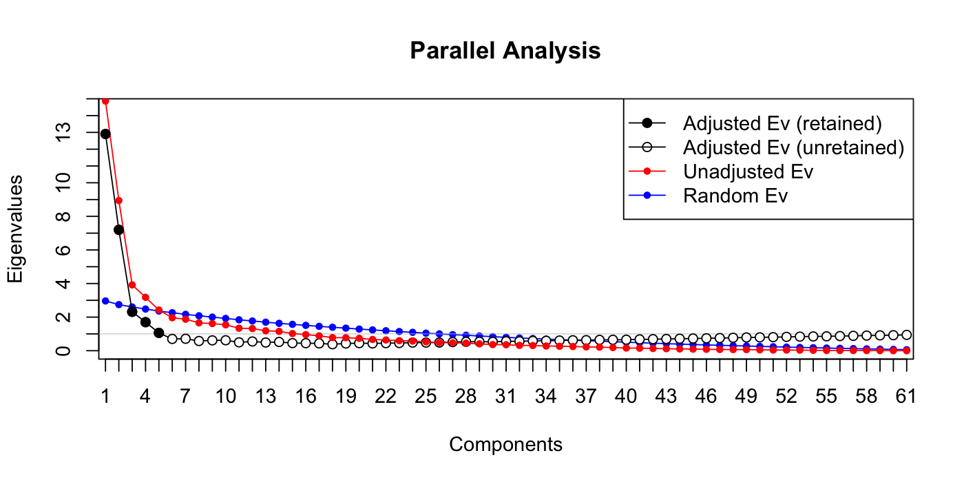
paran(votes_numeric[,vote_descriptions$category == "passage"], graph = TRUE, iterations = 100)

## 
## Using eigendecomposition of correlation matrix.
## Computing: 10%  20%  30%  40%  50%  60%  70%  80%  90%  100%
## 
## 
## Results of Horn's Parallel Analysis for component retention
## 100 iterations, using the mean estimate
## 
## -------------------------------------------------- 
## Component   Adjusted    Unadjusted    Estimated 
##             Eigenvalue  Eigenvalue    Bias 
## -------------------------------------------------- 
## 1          12.904483   14.866993      1.962509
## 2           7.196930    8.941067      1.744137
## 3           2.314958    3.918645      1.603687
## 4           1.698357    3.179481      1.481123
## 5           1.061265    2.422535      1.361270
## -------------------------------------------------- 
## 
## Adjusted eigenvalues > 1 indicate dimensions to retain.
## (5 components retained)

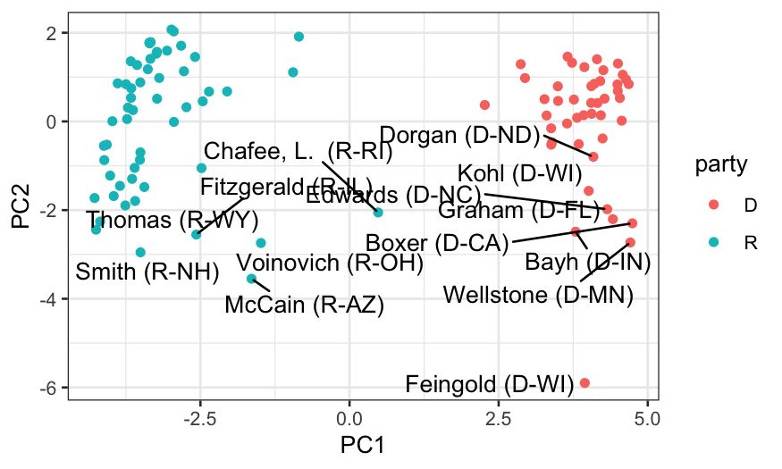
members_and_scores_passage = data.frame(members, out_prcomp_passage$x)
ggplot(members_and_scores_passage, aes(x = PC1, y = PC2)) +
    geom_point(aes(color = party)) +
    geom_text_repel(aes(label = display_name))

Looking at just the “procedural” votes

out_prcomp_procedural = prcomp(votes_numeric[,vote_descriptions$category == "procedural"])
plot(out_prcomp_procedural$sdev^2 / sum(out_prcomp_procedural$sdev^2),
     ylab = "Fraction of variance explained", xlab = "Component")

out_prcomp_procedural$sdev[1]^2 / sum(out_prcomp_procedural$sdev^2)

## [1] 0.670782

paran(votes_numeric[,vote_descriptions$category == "procedural"], graph = TRUE, iterations = 100)

## 
## Using eigendecomposition of correlation matrix.
## Computing: 10%  20%  30%  40%  50%  60%  70%  80%  90%  100%
## 
## 
## Results of Horn's Parallel Analysis for component retention
## 100 iterations, using the mean estimate
## 
## -------------------------------------------------- 
## Component   Adjusted    Unadjusted    Estimated 
##             Eigenvalue  Eigenvalue    Bias 
## -------------------------------------------------- 
## 1          93.440562   97.330067      3.889504
## 2           1.622993    5.285660      3.662667
## -------------------------------------------------- 
## 
## Adjusted eigenvalues > 1 indicate dimensions to retain.
## (2 components retained)

members_and_scores_procedural = data.frame(members, out_prcomp_procedural$x)
ggplot(members_and_scores_procedural, aes(x = PC1, y = PC2)) +
    geom_point(aes(color = party)) +
    geom_text_repel(aes(label = display_name))

What did we learn?

We always see one dimension that explains a very large fraction of the variance.

In both the votes overall and in the passage votes, we get five dimensions that have more information than we would expect if all the votes were uncorrelated with each other.

In just the procedural votes, the first dimension explains more of the variance and there are only two dimensions that have more information than we would expect if all the votes were uncorrelated with each other.

Overall

Important to look at the scree plot

Comparing to a null distribution can help with interpretation. Parallel analysis is probably the most useful, but you can also use the random matrix theory-based results as well.

Parallel analysis usually more accurate.

RMT results faster.