
Julia Fukuyama
Today: PCA
Suppose we have a 3-dimensional object that we want to investigate.
Due to some strange set of constraints, we are only allowed to see its shadow.
Without knowing anything about the object, what sort of a shadow would you expect to be most useful?


It seems like the most useful shadow is the biggest one: If we were only allowed one view, we would ask for the one that took up the most space.
It’s easy to come up with examples where this isn’t the most useful, but it’s a good place to start if you don’t know anything about the data.
The same will be true of PCA.
In PCA, we have a data matrix \(\mathbf X \in \mathbb R^{n \times p}\) with centered columns.
We think of the rows of \(\mathbf X\) as points in \(p\)-dimensional space, and we want to project the points down into a lower-dimensional space so we can visualize them.
There are a lot of different ways we could do this, but in PCA we want to find the projection that maximizes the variance of the projected points.
First consider projecting the points onto a line.
The PCA problem is to find \[ \mathbf w_{(1)} = \text{arg max}_{\mathbf w : \|\mathbf w \| = 1} \sum_{i=1}^n (\mathbf x_i \cdot \mathbf w)^2 \] where \(\mathbf x_i\) is the \(i\)th row of \(\mathbf X\).
\(\mathbf w_{(1)}\) is then the first principal component.
If we want projections into higher-dimensional spaces, we take more principal components.
We find the \(k\)th principal component as \[ \mathbf w_{(k)} = \text{arg max}_{\mathbf w :\| \mathbf w \| = 1, \mathbf w^T \mathbf w_{(j)} = 0, j = 1, \ldots, k-1} \sum_{i=1}^n (\mathbf x_i \cdot \mathbf w)^2 \]
The constraint that \(\mathbf w^T \mathbf w_{(k)} = 0, j = 1,\ldots, k-1\) means that the \(k\)th principal component is orthogonal to all the previous principal components, and is needed to ensure a unique solution to the problem.
The solution to the PCA is given by the SVD.
If \(\mathbf X\) has centered columns and \(\mathbf X = \mathbf U \mathbf D \mathbf V^T\) is the SVD of \(\mathbf X\), then
## Loading required package: plyr## Loading required package: scales## Loading required package: grid## Loading required package: viridisLite##
## Attaching package: 'viridis'## The following object is masked from 'package:scales':
##
## viridis_palOlympic dataset
##       100             long            poid            haut
##  Min.   :10.62   Min.   :6.220   Min.   :10.27   Min.   :1.790
##  1st Qu.:11.02   1st Qu.:7.000   1st Qu.:13.15   1st Qu.:1.940
##  Median :11.18   Median :7.090   Median :14.12   Median :1.970
##  Mean   :11.20   Mean   :7.133   Mean   :13.98   Mean   :1.983
##  3rd Qu.:11.43   3rd Qu.:7.370   3rd Qu.:14.97   3rd Qu.:2.030
##  Max.   :11.57   Max.   :7.720   Max.   :16.60   Max.   :2.270
##       400             110             disq            perc
##  Min.   :47.44   Min.   :14.18   Min.   :34.36   Min.   :4.000
##  1st Qu.:48.34   1st Qu.:14.72   1st Qu.:39.08   1st Qu.:4.600
##  Median :49.15   Median :15.00   Median :42.32   Median :4.700
##  Mean   :49.28   Mean   :15.05   Mean   :42.35   Mean   :4.739
##  3rd Qu.:49.98   3rd Qu.:15.38   3rd Qu.:44.80   3rd Qu.:4.900
##  Max.   :51.28   Max.   :16.20   Max.   :50.66   Max.   :5.700
##       jave            1500
##  Min.   :49.52   Min.   :256.6
##  1st Qu.:55.42   1st Qu.:266.4
##  Median :59.48   Median :272.1
##  Mean   :59.44   Mean   :276.0
##  3rd Qu.:64.00   3rd Qu.:286.0
## Max. :72.60 Max. :303.2## PC1 PC2
## 100 -0.0045042348 0.005632863
## long 0.0084964324 -0.013772028
## poid -0.0294931259 -0.155510542
## haut 0.0007153041 -0.002667193
## 400 -0.0455887408 -0.001324105
## 110 -0.0050441978 0.010836485
## disq -0.1184059716 -0.352166545
## perc 0.0003427802 -0.019704006
## jave -0.0525411029 -0.917592971
## 1500 -0.9900266310 0.095301595Two types of biplots, form and covariance. Let’s start off with the form biplot.
This allows us to read off the sample scores along the principal axes and the variable weights along the principal axes.
However, there’s another way to interpret the PCA biplot:
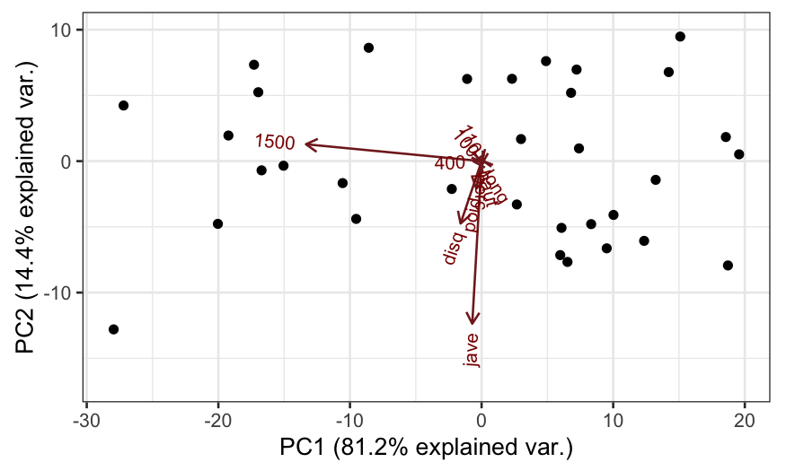
The covariance biplot is very subtly different from the form biplot, the difference being how the singular values are allocated.
In the covariance biplot, we use
In this form of the biplot, the angles between biplot axes and their lengths tell us about the covariances between variables.
Why is this?
Following up on what we talked about regarding correlations between variables, note the following two relationships:
Therefore, the columns of \(\mathbf V \mathbf D\) can be seen as giving us both biplot points and biplot axes for approximating the covariance matrix, and projections of one biplot axis onto another biplot axis tells us about the covariance between the two variables.
The example above suggests that doing PCA when the variables are on different scales isn’t always that useful.
When the variables are on different scales and measure different things, we often standardize the columns of \(\mathbf X\) (divide each column by its standard deviation) before performing PCA.
This is sometimes referred to as correlation-based PCA, as opposed to covariance-based PCA.
Analogous to the covariance-based PCA biplot:
Interpretation as a reduced-rank biplot:
Relationships between the variables:
Covariance PCA biplot based on correlations, with some extra information:
oly_scale = prcomp(olympic$tab, scale. = TRUE)
## scale = 1 means covariance biplot
ggbiplot(oly_scale, scale = 1)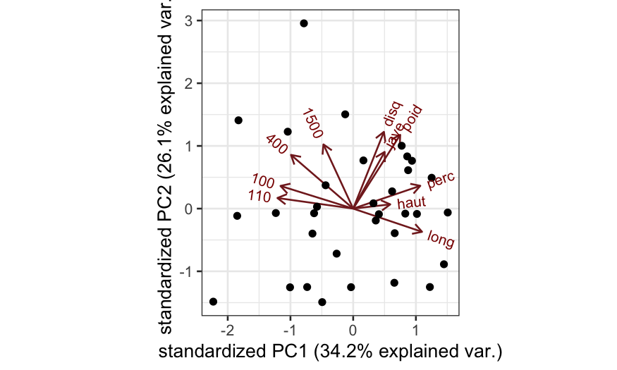
How would you interpret the first principal component?
Covariance PCA biplot based on correlations, with some extra information:
## scale = 1 means covariance biplot
ggbiplot(oly_scale, scale = 1) +
    geom_point(aes(color = olympic$score)) +
    scale_color_viridis("Score")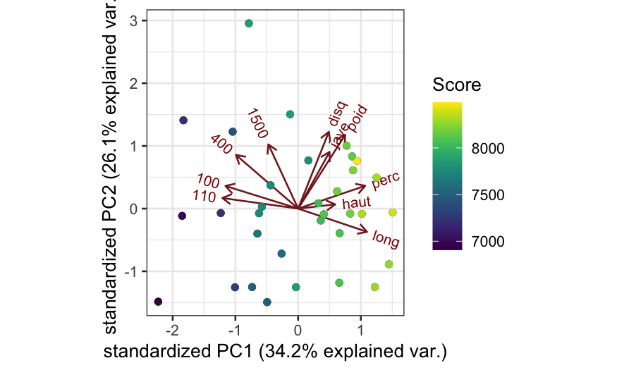
Wine dataset
# ggbiplot is not on cran, so you have to use
# library(devtools)
# install_github("vqv/ggbiplot")
library(ggbiplot)
data(wine)
nrow(wine)
## [1] 178## Alcohol MalicAcid Ash AlcAsh
## Min. :11.03 Min. :0.740 Min. :1.360 Min. :10.60
## 1st Qu.:12.36 1st Qu.:1.603 1st Qu.:2.210 1st Qu.:17.20
## Median :13.05 Median :1.865 Median :2.360 Median :19.50
## Mean :13.00 Mean :2.336 Mean :2.367 Mean :19.49
## 3rd Qu.:13.68 3rd Qu.:3.083 3rd Qu.:2.558 3rd Qu.:21.50
## Max. :14.83 Max. :5.800 Max. :3.230 Max. :30.00
## Mg Phenols Flav NonFlavPhenols
## Min. : 70.00 Min. :0.980 Min. :0.340 Min. :0.1300
## 1st Qu.: 88.00 1st Qu.:1.742 1st Qu.:1.205 1st Qu.:0.2700
## Median : 98.00 Median :2.355 Median :2.135 Median :0.3400
## Mean : 99.74 Mean :2.295 Mean :2.029 Mean :0.3619
## 3rd Qu.:107.00 3rd Qu.:2.800 3rd Qu.:2.875 3rd Qu.:0.4375
## Max. :162.00 Max. :3.880 Max. :5.080 Max. :0.6600
## Proa Color Hue OD
## Min. :0.410 Min. : 1.280 Min. :0.4800 Min. :1.270
## 1st Qu.:1.250 1st Qu.: 3.220 1st Qu.:0.7825 1st Qu.:1.938
## Median :1.555 Median : 4.690 Median :0.9650 Median :2.780
## Mean :1.591 Mean : 5.058 Mean :0.9574 Mean :2.612
## 3rd Qu.:1.950 3rd Qu.: 6.200 3rd Qu.:1.1200 3rd Qu.:3.170
## Max. :3.580 Max. :13.000 Max. :1.7100 Max. :4.000
## Proline
## Min. : 278.0
## 1st Qu.: 500.5
## Median : 673.5
## Mean : 746.9
## 3rd Qu.: 985.0
## Max. :1680.0## PC1 PC2
## Alcohol -0.144329395 -0.483651548
## MalicAcid 0.245187580 -0.224930935
## Ash 0.002051061 -0.316068814
## AlcAsh 0.239320405 0.010590502
## Mg -0.141992042 -0.299634003
## Phenols -0.394660845 -0.065039512
## Flav -0.422934297 0.003359812
## NonFlavPhenols 0.298533103 -0.028779488
## Proa -0.313429488 -0.039301722
## Color 0.088616705 -0.529995672
## Hue -0.296714564 0.279235148
## OD -0.376167411 0.164496193
## Proline -0.286752227 -0.364902832## PC1 PC2
## [1,] -3.307421 -1.4394023
## [2,] -2.203250 0.3324551
## [3,] -2.509661 -1.0282507
## [4,] -3.746497 -2.7486184
## [5,] -1.006070 -0.8673840
## [6,] -3.041674 -2.1164309
## [7,] -2.442201 -1.1715453
## [8,] -2.053644 -1.6044371
## [9,] -2.503811 -0.9154885
## [10,] -2.745882 -0.7872170principal_axes = data.frame(wine.pca$rotation)
scores = data.frame(wine.pca$x)
ggplot(principal_axes) + geom_segment(aes(x = PC1, y = PC2, xend = 0, yend = 0))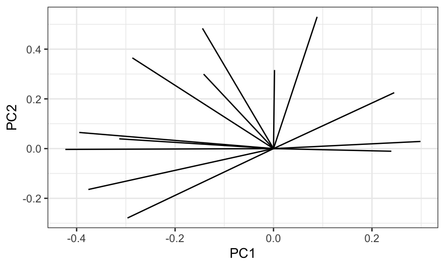
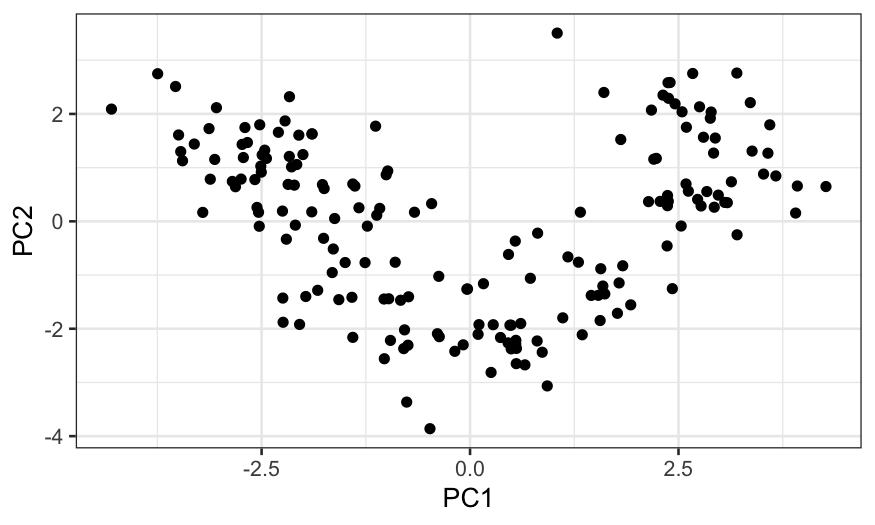
Interpretation of PCA:
Two kinds of PCA:
scale. = FALSE in
prcomp (the default)scale. = TRUE in
prcompTwo kinds of PCA biplot:
scale = 0 in
ggbiplotscale = 1 in
ggbiplot