Stat 470/670 Lecture 22: Matrix Approximation, the
SVD, and Reduced Rank Biplots
Julia Fukuyama
Today
- Singular Value Decomposition
Reading: Greenacre, Biplots in Practice, Chapter 5. The book
website contains links to all the chapters. Also here.
What to know about biplots
- A biplot is a generalization of a scatterplot to an arbitrary number
of variables.
- The value of each observation for each variable is read off of the
biplot by projecting the point onto the variable “axis”, just as in a
scatterplot.
- We can represent a matrix \(\mathbf S \in
\mathbb R^{n \times p}\) as a biplot if we can write \(\mathbf S = \mathbf L \mathbf R^T\), where
\(\mathbf L \in \mathbb R^{n \times
2}\) and \(\mathbf R \in \mathbb R^{p
\times 2}\).
Rank of a matrix
One more concept from linear algebra:
The rank of a matrix is the maximum number of linearly
independent rows or columns of a matrix.
- A set of vectors \(\mathbf v_1, \ldots,
\mathbf v_n\) is linearly dependent if there exist a set
of scalar values \(a_1, \ldots, a_n\)
such that \(\sum_{i=1}^n a_i \mathbf v_i =
\mathbf 0\), where \(\mathbf 0\)
represents the vector containing all zero values.
- A set of vectors \(\mathbf v_1, \ldots,
\mathbf v_n\) is linearly independent if it is not
linearly dependent.
Note: If you’ve had linear algebra this should be familiar to you. If
you haven’t had linear algebra or don’t particularly remember about
ranks that’s ok too, the main idea here is going to be that the rank of
a matrix controls whether we can represent it exactly in two dimensions
or not.
Properties of the rank:
- The rank is well defined, for any matrix the number of linearly
independent rows and the number of linearly independent columns is the
same.
- An \(n \times p\) matrix has rank
at most \(\text{min}(n, p)\).
- If a matrix \(\mathbf S \in \mathbb R^{n
\times p}\) has rank \(k\),
there exist matrices \(\mathbf L \in \mathbb
R^{n \times k}\) and \(\mathbf R \in
\mathbb R^{p \times k}\) such that \(\mathbf S = \mathbf L \mathbf R^T\).
Problem we need to solve to make a biplot of a high-dimensional
matrix
Suppose we have a matrix \(\mathbf S \in
\mathbb R^{n \times p}\), and \(\mathbf
S\) has rank greater than 2.
To make a biplot, we need to have \(\mathbf
S = \mathbf L \mathbf R^T\), where \(\mathbf L \in \mathbb R^{n \times 2}\) and
\(\mathbf R \in \mathbb R^{p \times
2}\).
If the rank if \(\mathbf S\) is more
than 2, such matrices don’t exist!
Solution: Find the rank-2 matrix \(\hat
{\mathbf S}\) that most closely approximates \(\mathbf S\), and use that to make a
biplot.
\[
\hat {\mathbf S} = \text{argmin}_{\mathbf T : \text{rank}(\mathbf T) =
2} \sum_{i=1}^n \sum_{j=1}^p (\mathbf S_{ij} - \mathbf T_{ij})^2
\]
Singular Value Decomposition
The Singular
Value Decomposition (SVD) is one of the most useful matrix
decompositions.
It says that any matrix \(\mathbf
S\) of rank \(r\) can be written
as \[
\mathbf S = \mathbf U \mathbf D \mathbf V^T
\] where:
- \(\mathbf U \in \mathbb R^{n \times
r}\), with orthogonal columns (the scalar product between any two
distinct columns is 0, the scalar product between any column and itself
is 1).
- \(\mathbf D \in \mathbb R^{r \times
r}\) is a diagonal matrix, with positive numbers on the diagonal.
These are written in decreasing order.
- \(\mathbf V \in \mathbb R^{p \times
r}\), with orthogonal columns.
Matrix Approximation by the SVD
We can use the SVD to find the solution to our problem on the
previous slide:
We want \(\hat{\mathbf S}\) such
that \[
\hat {\mathbf S} = \text{argmin}_{\mathbf T : \text{rank}(\mathbf T) =
2} \sum_{i=1}^n \sum_{j=1}^p (\mathbf S_{ij} - \mathbf T_{ij})^2
\]
It turns out that \(\hat{\mathbf S} =
\mathbf U_{(2)} \mathbf D_{(2)} \mathbf V_{(2)}^T\), where
- \(\mathbf U_{(2)} \in \mathbb R^{n \times
2}\) is the matrix containing the first two columns of the matrix
\(\mathbf U\) in the SVD of \(\mathbf S\)
- \(\mathbf D_{(2)} \in \mathbb R^{2 \times
2}\) is the diagonal matrix containing the first two rows and
columns of \(\mathbf D\) in the SVD of
\(\mathbf S\).
- \(\mathbf V_{(2)} \in \mathbb R^{p \times
2}\) is the matrix containing the first two columns of the matrix
\(\mathbf V\) in the SVD of \(\mathbf S\)
Quality of the approximation
The values in \(\mathbf D\) tell us
about how well \(\hat {\mathbf S}\)
approximates \(\mathbf S\).
We have
\[
1 - \frac{\mathbf D_{11}^2 + \mathbf D_{22}^2}{\sum_{i=1}^r \mathbf
D_{ii}^2} = \frac{\sum_{i=1}^n \sum_{j=1}^p (\hat {\mathbf S}_{ij} -
\mathbf S_{ij})^2}{\sum_{i=1}^n \sum_{j=1}^p \mathbf S_{ij}^2}
\]
This is the quality of a rank-2 approximation because we are
interested in biplots and representations of \(\mathbf S\) in the plane, but the analogous
result holds for approximations of any rank.
Biplot representation of the SVD approximation
\(\hat{\mathbf S} = \mathbf U_{(2)} \mathbf
D_{(2)} \mathbf V_{(2)}^T\) is almost in the right form for a
biplot, but not quite. We need just a left and a right matrix, and we
have \(\mathbf D_{(2)}\) in the
middle.
We have a couple of options:
- Left matrix \(\mathbf U_{(2)}\),
right matrix \(\mathbf V_{(2)} \mathbf
D_{(2)}\)
- Left matrix \(\mathbf U_{(2)} \mathbf
D_{(2)}\), right matrix \(\mathbf
V_{(2)}\)
- Left matrix \(\mathbf U_{(2)} \mathbf
D_{(2)}^{1/2}\), right matrix \(\mathbf
V_{(2)} \mathbf D_{(2)}^{1/2}\)
The last is referred to as the symmetric biplot, and we’ll go with
that for now.
Example
## HairEyeColor dataset, we'll just use the women
HairEyeColor
## , , Sex = Male
##
##        Eye
## Hair    Brown Blue Hazel Green
##   Black    32   11    10     3
##   Brown    53   50    25    15
##   Red      10   10     7     7
##   Blond     3   30     5     8
##
## , , Sex = Female
##
##        Eye
## Hair    Brown Blue Hazel Green
##   Black    36    9     5     2
##   Brown    66   34    29    14
##   Red      16    7     7     7
##   Blond     4   64     5     8
hec_svd = svd(HairEyeColor[,,2])
hec_svd
## $d
## [1] 98.392552 52.703025  9.489478  3.201033
##
## $u
##            [,1]       [,2]       [,3]        [,4]
## [1,] -0.3341488  0.3032153  0.8780094  0.15970129
## [2,] -0.7993476  0.3549164 -0.3697302 -0.31365176
## [3,] -0.1921516  0.1032077 -0.2788792  0.93522849
## [4,] -0.4609401 -0.8783183  0.1209359  0.03828508
##
## $v
##            [,1]        [,2]       [,3]        [,4]
## [1,] -0.7084325  0.61625080  0.3401477  0.05155421
## [2,] -0.6202744 -0.77213448  0.1179200 -0.07185294
## [3,] -0.2896722  0.15444110 -0.8092755 -0.48714583
## [4,] -0.1716771 -0.01382906 -0.4641847  0.86883155
## Quality of the rank-2 approximation:
sum(hec_svd$d[1:2]^2) / sum(hec_svd$d^2)
## [1] 0.9920139
## Distribute the singular values evenly between the left and right singular vectors
left_matrix = hec_svd$u[,1:2] %*% diag(hec_svd$d[1:2]^(.5))
right_matrix = hec_svd$v[,1:2] %*% diag(hec_svd$d[1:2]^(.5))
Let’s check the quality of the approximations
##        Eye
## Hair    Brown Blue Hazel Green
##   Black    36    9     5     2
##   Brown    66   34    29    14
##   Red      16    7     7     7
##   Blond     4   64     5     8
round(left_matrix %*% t(right_matrix), digits = 1)
##      [,1] [,2] [,3] [,4]
## [1,] 33.1  8.1 12.0  5.4
## [2,] 67.2 34.3 25.7 13.2
## [3,] 16.7  7.5  6.3  3.2
## [4,]  3.6 63.9  6.0  8.4
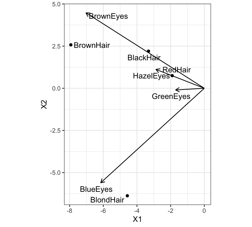
Set up for making a biplot:
## Change the matrices to data frames and add a column describing the variables
left_df = data.frame(left_matrix, HairColor = paste0(rownames(HairEyeColor), "Hair"))
right_df = data.frame(right_matrix, EyeColor = paste0(colnames(HairEyeColor), "Eyes"))
##          X1         X2 HairColor
## 1 -3.314523  2.2012479 BlackHair
## 2 -7.928970  2.5765809 BrownHair
## 3 -1.906010  0.7492551   RedHair
## 4 -4.572204 -6.3763140 BlondHair
##          X1         X2  EyeColor
## 1 -7.027156  4.4737866 BrownEyes
## 2 -6.152689 -5.6054530  BlueEyes
## 3 -2.873346  1.1211937 HazelEyes
## 4 -1.702917 -0.1003946 GreenEyes
ggplot(left_df) + geom_text_repel(aes(x = X1, y = X2, label = HairColor)) +
    geom_point(aes(x = X1, y = X2)) +
    coord_fixed() +
    geom_segment(aes(xend = X1, yend = X2, x = 0, y = 0),
                 data = right_df, arrow = arrow(length = unit(0.03, "npc"))) +
    geom_text_repel(aes(x = X1, y = X2, label = EyeColor), data = right_df)

We can look at what happens the other way as well:
## Distribute the singular values only to the right singular vectors
left_matrix = hec_svd$u[,1:2]
right_matrix = hec_svd$v[,1:2] %*% diag(hec_svd$d[1:2])
Let’s check the quality of the approximations
##        Eye
## Hair    Brown Blue Hazel Green
##   Black    36    9     5     2
##   Brown    66   34    29    14
##   Red      16    7     7     7
##   Blond     4   64     5     8
round(left_matrix %*% t(right_matrix), digits = 1)
##      [,1] [,2] [,3] [,4]
## [1,] 33.1  8.1 12.0  5.4
## [2,] 67.2 34.3 25.7 13.2
## [3,] 16.7  7.5  6.3  3.2
## [4,]  3.6 63.9  6.0  8.4
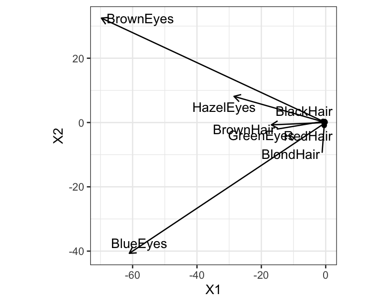
Set up for making a biplot:
## Change the matrices to data frames and add a column describing the variables
left_df = data.frame(left_matrix, HairColor = paste0(rownames(HairEyeColor), "Hair"))
right_df = data.frame(right_matrix, EyeColor = paste0(colnames(HairEyeColor),"Eyes"))
##           X1         X2 HairColor
## 1 -0.3341488  0.3032153 BlackHair
## 2 -0.7993476  0.3549164 BrownHair
## 3 -0.1921516  0.1032077   RedHair
## 4 -0.4609401 -0.8783183 BlondHair
##          X1          X2  EyeColor
## 1 -69.70448  32.4782811 BrownEyes
## 2 -61.03038 -40.6938228  BlueEyes
## 3 -28.50159   8.1395131 HazelEyes
## 4 -16.89175  -0.7288331 GreenEyes
ggplot(left_df) + geom_text_repel(aes(x = X1, y = X2, label = HairColor)) +
    geom_point(aes(x = X1, y = X2)) +
    coord_fixed() +
    geom_segment(aes(xend = X1, yend = X2, x = 0, y = 0),
                 data = right_df, arrow = arrow(length = unit(0.03, "npc"))) +
    geom_text_repel(aes(x = X1, y = X2, label = EyeColor), data = right_df)

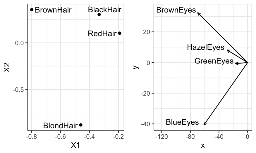
p1 = ggplot(left_df) + geom_text_repel(aes(x = X1, y = X2, label = HairColor)) +
    geom_point(aes(x = X1, y = X2))

p2 = ggplot(right_df) +
    geom_segment(aes(xend = X1, yend = X2, x = 0, y = 0), arrow = arrow(length = unit(0.03, "npc"))) +
    geom_text(aes(x = X1, y = X2, label = EyeColor), nudge_y = 2, nudge_x = -30) + xlim(c(-125, 0))
multiplot(p1, p2, cols = 2)

Overall:
- Not every matrix can be written as the product of two two-column
matrices.
- The SVD gives us the best approximation in terms of MSE.
- We have some freedom in how to make the biplot based on the
SVD.
- Notice that there is no estimation here: we are trying to represent
the matrix, both the signal and the noise.
