Vectors and Matrices

A vector in $\mathbb R^n$ is given by a set of $n$ coordinates. We will write a vector $\mathbf x \in \mathbb R^n$ as $(x_1, x_2, \ldots, x_n)$.

We think of vectors in $\mathbb R^2$ as points in the plane, vectors in $\mathbb R^3$ as points in 3-dimensional space, and vectors in $\mathbb R^n$ as points in $n$-dimensional space.

A matrix in $\mathbb R^{n \times p}$ consists of $n$ rows and $p$ columns. We will write such a matrix as \[ \mathbf X = \begin{pmatrix} \mathbf X_{11} & \mathbf X_{12} & \cdots & \mathbf X_{1p} \\ \mathbf X_{21} & \mathbf X_{22} & \cdots & \mathbf X_{2p} \\ \vdots & \vdots & \ddots & \vdots \\ \mathbf X_{n1} & \mathbf X_{n2} & \cdots & \mathbf X_{np} \end{pmatrix} \] so that $\mathbf X_{ij}$ represents the element in the $i$th row and $j$th column of $\mathbf X$.

A column vector is a vector written as an $n \times 1$ matrix, and a row vector is a vector written as a $1 \times n$ matrix.

Scalar products

Suppose $\mathbf x$ and $\mathbf y$ are vectors in $\mathbb R^n$, then the scalar product of $\mathbf x$ and $\mathbf y$ is \[ \mathbf x \cdot \mathbf y = \sum_{i=1}^n x_i y_i \]

Norm of a vector

Suppose $\mathbf x$ is a vector in $\mathbb R^n$. The norm of $\mathbf x$ is defined as \[ \| \mathbf x\| = \sqrt{\sum_{i=1}^n x_i^2} \]

The norm is usually interpreted as a measure of size or length.

Vector operation properties

$\frac{\mathbf x \cdot \mathbf y }{ \|\mathbf x\| \|\mathbf y\|} = \cos(\theta)$, where $\theta$ is the angle between $\mathbf x$ and $\mathbf y$.
$\mathbf x \cdot \mathbf y = 0$ means that $\mathbf x$ and $\mathbf y$ are orthogonal, i.e. that the angle between them is 90 degrees.
If $\|\mathbf x\| = 1$ and $\|\mathbf y\| = 1$ (referred to as unit vectors), then $\mathbf x \cdot \mathbf y \in [-1, 1]$.
If $\mathbf x$ and $\mathbf y$ are unit vectors, then $\mathbf x \cdot \mathbf y = 1$ implies the angle between the two vectors is $0$, and $\mathbf x \cdot \mathbf y = -1$ implies that the angle between the two vectors is $180$ degrees. This property motivates the interpretation of the scalar product as a measure of similarity.

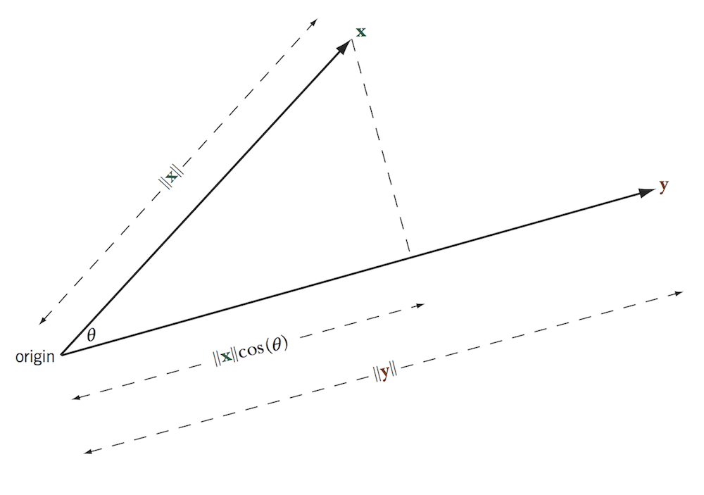
Geometry: Projection of one vector onto another

The length of the projection of $\mathbf x$ onto $\mathbf y$ is $\|\mathbf x \| \cos(\theta) = (\mathbf x \cdot \mathbf y) / \|\mathbf y\|$.

More useful form: \[ \mathbf x \cdot \mathbf y = (\text{length of projection of $\mathbf x$ onto $\mathbf y$})\|\mathbf y\| \]

This result is important for visualization because we can “read off” scalar products as projections.

Matrix operations: Multiplication

Suppose $\mathbf X \in \mathbb R^{a \times b}$ and $\mathbf Y \in \mathbb R^{b \times c}$. Then the matrix product of $\mathbf X$ and $\mathbf Y$ is a matrix $\mathbf S \in \mathbb R^{a \times c}$, where the $i, j$ element of $\mathbf S$ is \[ \mathbf S_{ij} = \sum_{k=1}^ b \mathbf X_{i k} \mathbf Y_{k j} \]

Note: For the matrix multiplication operation to be defined for the matrices $\mathbf X$ and $\mathbf Y$, the number of columns of $\mathbf X$ must be equal to the number of rows of $\mathbf Y$.

Matrix operations: Transpose

The matrix transpose operation flips the row and column indices. That is, $(\mathbf X^T)_{ij} = \mathbf X_{ji}$.

Matrix multiplication written as scalar products

Note that we can write the matrix multiplication operation in terms of scalar products.

As before, suppose we have $\mathbf X \in \mathbb R^{a \times b}$ and $\mathbf Y \in \mathbb R^{b \times c}$.

Let $\mathbf x_1, \ldots, \mathbf x_a$ be column vectors containing the rows of $\mathbf X$, so that \[ \mathbf X = \begin{pmatrix} \mathbf x_1^T \\ \vdots \\ \mathbf x_a^T \end{pmatrix} \] and let $\mathbf y_1, \ldots, \mathbf y_c$ be column vectors containing the columns of $\mathbf Y$, so that \[ \mathbf Y = \begin{pmatrix} \mathbf y_1 & \cdots & \mathbf y_c \end{pmatrix} \]

Then if $\mathbf S = \mathbf X \mathbf Y$, $\mathbf S_{ij} = \mathbf x_i \cdot \mathbf y_j$.

\[ \mathbf S = \begin{pmatrix} \mathbf x_1 \cdot \mathbf y_1 & \mathbf x_1 \cdot \mathbf y_2 & \cdots & \mathbf x_1 \cdot \mathbf y_c\\ \mathbf x_2 \cdot \mathbf y_1& \mathbf x_2 \cdot \mathbf y_2 & \cdots & \mathbf x_2 \cdot \mathbf y_c\\ \vdots & \vdots & \ddots & \vdots \\ \mathbf x_a \cdot \mathbf y_1& \mathbf x_a \cdot \mathbf y_2& \cdots & \mathbf x_a \cdot \mathbf y_c \end{pmatrix} \]

Biplot: the main idea

Suppose we have a matrix $\mathbf S \in \mathbb R^{n \times p}$.

The rows of $\mathbf S$ correspond to observations, and the columns of $\mathbf S$ correspond to the variables measured.

A biplot is a visualization of the matrix $\mathbf S$ that will allow us to read off

The values of $\mathbf S$,

(In some cases) the similarities between the variables,

(In most cases) the similarities between the observations.

To do this, we combine our results about matrix multiplication as scalar products with our results describing scalar products in terms of projections of one variable onto another.

Biplot definition

Suppose we have a matrix $\mathbf S \in \mathbb R^{n \times p}$. Further suppose that we can write $\mathbf S$ as \[ \mathbf S = \mathbf X \mathbf Y^T, \] where $\mathbf X \in \mathbb R^{n \times 2}$ and $\mathbf Y \in \mathbb R^{p \times 2}$.

$\mathbf S$ is the target matrix, and $\mathbf X$ and $\mathbf Y$ are the left and right matrices, respectively.

In a biplot, we plot the rows of $\mathbf X$ and the rows of $\mathbf Y$.

The convention is that

Rows of $\mathbf X$ are plotted as points, and are referred to as biplot points.

Rows of $\mathbf Y$ are plotted as arrows, and are referred to as biplot vectors.

Example 1: A scatterplot

Suppose we have a matrix $\mathbf X$ with $n$ rows and 2 columns.

We can write \[ \mathbf X = \mathbf X \begin{pmatrix} 1 & 0 \\ 0 & 1 \end{pmatrix} \] which is the form we need for a biplot.

Example 2: Something more complicated

X = matrix(c(2,2, 1,2, -1,1, 1,-1, 2,-2), ncol = 2, byrow = TRUE)
Y = matrix(c(3,1, 2,-1, -1,2, -2,-1), ncol = 2, byrow = TRUE)
## %*% is the matrix multiplication function in R
S = X %*% t(Y)
X

##      [,1] [,2]
## [1,]    2    2
## [2,]    1    2
## [3,]   -1    1
## [4,]    1   -1
## [5,]    2   -2

##      [,1] [,2]
## [1,]    3    1
## [2,]    2   -1
## [3,]   -1    2
## [4,]   -2   -1

##      [,1] [,2] [,3] [,4]
## [1,]    8    2    2   -6
## [2,]    5    0    3   -4
## [3,]   -2   -3    3    1
## [4,]    2    3   -3   -1
## [5,]    4    6   -6   -2

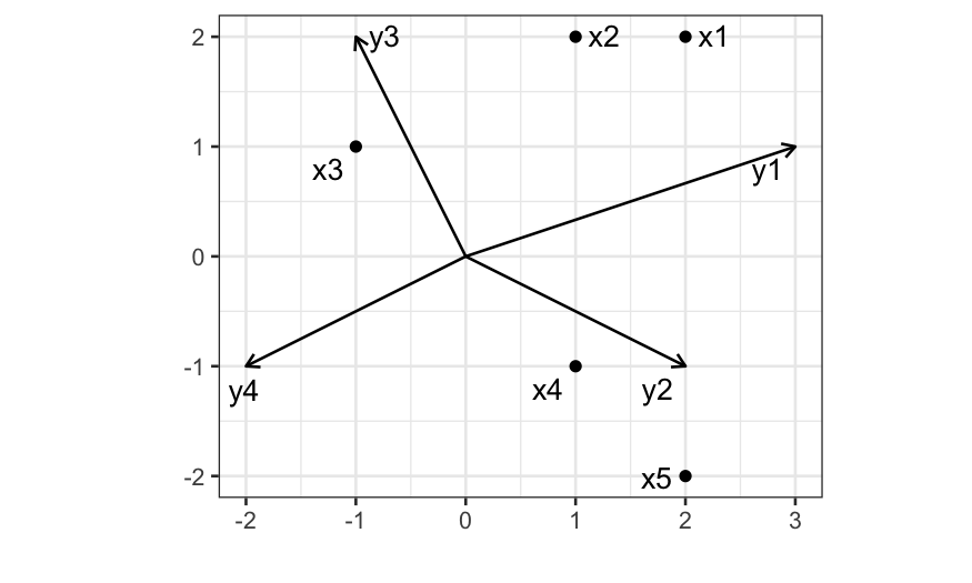
A toy biplot

The arrows are the biplot vectors, or the rows of $\mathbf Y$.

The points are the byplot points, or the rows of $\mathbf X$.

How do we use this plot?

We can read off the elements of the original data matrix

Remember that we can write S as a matrix of scalar products. \[ \mathbf S = \mathbf X \mathbf Y^T = \begin{pmatrix} \mathbf x_1 \cdot \mathbf y_1 & \mathbf x_1 \cdot \mathbf y_2 & \cdots & \mathbf x_1 \cdot \mathbf y_p \\ \mathbf x_2 \cdot \mathbf y_1 & \mathbf x_2 \cdot \mathbf y_2 & \cdots & \mathbf x_2 \cdot \mathbf y_p \\ \vdots & \vdots & \ddots & \vdots\\ \mathbf x_n \cdot \mathbf y_1 & \mathbf x_n \cdot \mathbf y_2 & \cdots & \mathbf x_n \cdot \mathbf y_p \end{pmatrix} \] where $\mathbf x_i$ are vectors denoting the rows of $\mathbf X$ and $\mathbf y_i$ are vectors denoting the rows of $\mathbf Y$

What this means is that we can reconstruct any element of S by looking at the scalar product between the biplot point and the biplot vector corresponding to that element.

Remember that the scalar product between $\mathbf x_i$ and $\mathbf y_j$ is the length of the projection of $\mathbf x_i$ onto $\mathbf y_j$ times the length of $\mathbf y_j$.

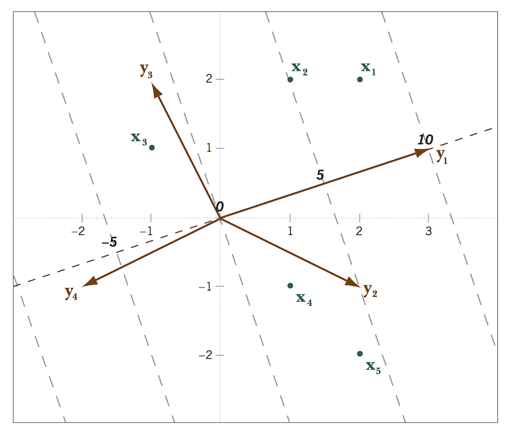
Biplot calibration

To read off absolute values, not just relative values, we need to calibrate the axes.

Suppose we are interested in the value in the target matrix for observation $i$, variable $j$.

Recall that \[ \text{length of the projection of point $\mathbf x_i$ onto vector $\mathbf y_j$} = (\mathbf x_i \cdot \mathbf y_j) /\|\mathbf y_j\|, \] and the value of the target matrix is \[ \mathbf S_{ij} = \mathbf x_i \cdot \mathbf y_j \]

Therefore, if the value in the target matrix is $1$, the length of the projection of $\mathbf x_i$ onto $\mathbf y_j$ is $1 / \|\mathbf y\|$. This is the length of one unit along the biplot axis, and it tells us that

If the biplot vector is long, the intervals between units on the biplot vector are short (and so values change quickly as we move along that axis).

If the biplot vector is short, the intervals between units on the biplot vector are long (and so values change slowly as we move along that axis).

Summing up

Think of a biplot as a generalization of a scatterplot. In a scatterplot, you visualize two variables. Points represent observations, and you can read off the value each variable takes for each observation. In biplots, we can have as many variables as we want; we are no longer limited to two.

However….

We can’t always write our data matrix as the product of two matrices with only two columns. What do we do in the general case?

Stat 470/670 Lecture 21: Background for Hypervariate Data

Today