Stat 470/670 Lecture 14: Model-building with a moderate number of variables

Julia Fukuyama

Model building

Over the next couple of weeks we’ll get back to building models, and we’ll look at models for different kinds of responses (binary, count, categorical).

Today we’ll look at model-building with a moderate number of variables. Today will be linear models, but the ideas carry over to logistic regression and the generalized linear models we’ll talk about later.

Note on terminology: for statisticians, “linear model” means that your response variable follows a normal distribution. “Generalized linear models” will be models for which the response variable follows a different sort of distribution.

Data: Prostate Cancer

We have a data set containing clinical data on patients who were about to receive a radical prostatectomy. The relevant variables are:

Variables about sizes:

lcavol: log cancer volume

lweight: log prostate weight

lbph: log of the amount of benign prostatic hyperplasia

Variables about the individual:

age: Age in years

Variables measured by the pathologist:

svi: Seminal vesicle invasion, a measure of how advanced the cancer is.

lcp: log of capsular penetration

gleason: A numeric vector giving the Gleason score. In theory can range from 2-10, in practice ranges from 6-10.

pgg45: Percent of cells with Gleason score 4 or 5.

The “response” variable:

lpsa: log of the concentration of prostate-stimulating antigen.

We are primarily interested in lpsa, which is used as a marker for prostate cancer. We would like to know whether and how it is related to the other variables we have available to us.

First we look at the data

prostate = read.table("../../datasets/prostate.txt")
summary(prostate)

##      lcavol           lweight           age             lbph        
##  Min.   :-1.3471   Min.   :2.375   Min.   :41.00   Min.   :-1.3863  
##  1st Qu.: 0.5128   1st Qu.:3.376   1st Qu.:60.00   1st Qu.:-1.3863  
##  Median : 1.4469   Median :3.623   Median :65.00   Median : 0.3001  
##  Mean   : 1.3500   Mean   :3.629   Mean   :63.87   Mean   : 0.1004  
##  3rd Qu.: 2.1270   3rd Qu.:3.876   3rd Qu.:68.00   3rd Qu.: 1.5581  
##  Max.   : 3.8210   Max.   :4.780   Max.   :79.00   Max.   : 2.3263  
##       svi              lcp             gleason          pgg45       
##  Min.   :0.0000   Min.   :-1.3863   Min.   :6.000   Min.   :  0.00  
##  1st Qu.:0.0000   1st Qu.:-1.3863   1st Qu.:6.000   1st Qu.:  0.00  
##  Median :0.0000   Median :-0.7985   Median :7.000   Median : 15.00  
##  Mean   :0.2165   Mean   :-0.1794   Mean   :6.753   Mean   : 24.38  
##  3rd Qu.:0.0000   3rd Qu.: 1.1787   3rd Qu.:7.000   3rd Qu.: 40.00  
##  Max.   :1.0000   Max.   : 2.9042   Max.   :9.000   Max.   :100.00  
##       lpsa           train        
##  Min.   :-0.4308   Mode :logical  
##  1st Qu.: 1.7317   FALSE:30       
##  Median : 2.5915   TRUE :67       
##  Mean   : 2.4784                  
##  3rd Qu.: 3.0564                  
##  Max.   : 5.5829

prostate = prostate %>% select(-"train")
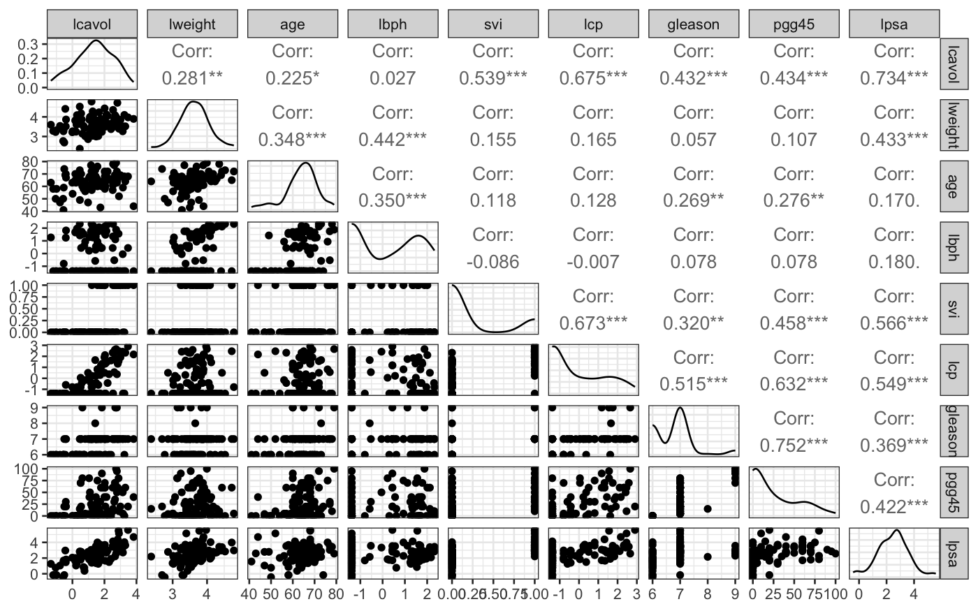
ggpairs(prostate, progress = FALSE)

From the ggpairs plot, we see that the distributions of the variables are reasonably symmetrical, not that skewed, and that there is at least some relationship between most of the variables and lpsa.

And a side note: this data set has already been transformed for you. Many of the variables are logged versions of what were presumably the raw measurements. This is actually a really important step: models with the logged variables perform substantially better than models with the raw variables, as we can see if we un-transform:

prostate_unlogged = prostate %>%
    mutate(cavol = exp(lcavol), weight = exp(lweight), bph = exp(lbph), cp = exp(lcp)) %>%
    select(-"lcavol", -"lweight", -"lbph", -"lcp")
summary(lm(lpsa ~ ., data = prostate))

## 
## Call:
## lm(formula = lpsa ~ ., data = prostate)
## 
## Residuals:
##      Min       1Q   Median       3Q      Max 
## -1.76644 -0.35510 -0.00328  0.38087  1.55770 
## 
## Coefficients:
##              Estimate Std. Error t value Pr(>|t|)    
## (Intercept)  0.181561   1.320568   0.137  0.89096    
## lcavol       0.564341   0.087833   6.425 6.55e-09 ***
## lweight      0.622020   0.200897   3.096  0.00263 ** 
## age         -0.021248   0.011084  -1.917  0.05848 .  
## lbph         0.096713   0.057913   1.670  0.09848 .  
## svi          0.761673   0.241176   3.158  0.00218 ** 
## lcp         -0.106051   0.089868  -1.180  0.24115    
## gleason      0.049228   0.155341   0.317  0.75207    
## pgg45        0.004458   0.004365   1.021  0.31000    
## ---
## Signif. codes:  0 '***' 0.001 '**' 0.01 '*' 0.05 '.' 0.1 ' ' 1
## 
## Residual standard error: 0.6995 on 88 degrees of freedom
## Multiple R-squared:  0.6634, Adjusted R-squared:  0.6328 
## F-statistic: 21.68 on 8 and 88 DF,  p-value: < 2.2e-16

summary(lm(lpsa ~ ., data = prostate_unlogged))

## 
## Call:
## lm(formula = lpsa ~ ., data = prostate_unlogged)
## 
## Residuals:
##      Min       1Q   Median       3Q      Max 
## -1.78876 -0.40705 -0.00634  0.46725  1.82792 
## 
## Coefficients:
##              Estimate Std. Error t value Pr(>|t|)    
## (Intercept)  0.759219   1.210444   0.627  0.53214    
## age         -0.008545   0.012087  -0.707  0.48144    
## svi          0.769166   0.270646   2.842  0.00557 ** 
## gleason      0.130183   0.166701   0.781  0.43694    
## pgg45        0.005412   0.004567   1.185  0.23927    
## cavol        0.073661   0.014479   5.087 2.03e-06 ***
## weight       0.012511   0.005322   2.351  0.02095 *  
## bph          0.056512   0.034547   1.636  0.10546    
## cp          -0.040047   0.034216  -1.170  0.24499    
## ---
## Signif. codes:  0 '***' 0.001 '**' 0.01 '*' 0.05 '.' 0.1 ' ' 1
## 
## Residual standard error: 0.764 on 88 degrees of freedom
## Multiple R-squared:  0.5985, Adjusted R-squared:  0.562 
## F-statistic:  16.4 on 8 and 88 DF,  p-value: 1.329e-14

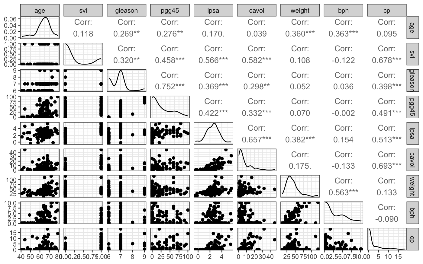
If we had started off with the raw data, we would have seen that we should log-transform some of the variables by looking at their marginal distributions: the variables that were transformed started off quite skewed, and the transformation got rid of the skewness.

ggpairs(prostate_unlogged, progress = FALSE)

Linear model with all the predictors

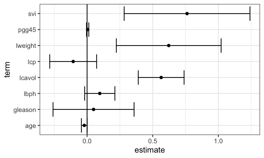
As a first step, we can fit a linear model with all the predictors and look at the results. We see that a lot of the coefficients are within the margin of error of zero, which suggests to us that a model with fewer predictors would do better.

prostate_lm = lm(lpsa ~ ., data = prostate)
prostate_coefs = tidy(prostate_lm, conf.int = TRUE)
ggplot(prostate_coefs[-1, ], aes(x = estimate, y = term, xmin = conf.low, xmax = conf.high)) +
    geom_point() + geom_errorbarh() + geom_vline(xintercept = 0)

Automatic ways of choosing subsets of variables

There are a lot of ways of doing variable selection for linear models.

Forward stepwise regression: Predictors are added to the model one at a time, stopping when adding a new predictor doesn’t seem to help. Computationally efficient.

Backward stepwise regression: Predictors are added to or subtracted from the model one at a time, stopping when subtracting an existing predictor seems to hurt too much (for backward stepwise). Works if you have fewer predictors than observations. Computationally efficient.

Best subsets: For every potential number of predictors used in the model, find the combination of predictors that does the best. Computationally intensive.

With eight predictors and a laptop, we can actually just look through all the subsets and see which model performs best.

This is what the regsubsets in the package leaps does for you.

library(leaps)
prostate_best_subset = regsubsets(lpsa ~ ., data = prostate)
summary(prostate_best_subset)$which

##   (Intercept) lcavol lweight   age  lbph   svi   lcp gleason pgg45
## 1        TRUE   TRUE   FALSE FALSE FALSE FALSE FALSE   FALSE FALSE
## 2        TRUE   TRUE    TRUE FALSE FALSE FALSE FALSE   FALSE FALSE
## 3        TRUE   TRUE    TRUE FALSE FALSE  TRUE FALSE   FALSE FALSE
## 4        TRUE   TRUE    TRUE FALSE  TRUE  TRUE FALSE   FALSE FALSE
## 5        TRUE   TRUE    TRUE  TRUE  TRUE  TRUE FALSE   FALSE FALSE
## 6        TRUE   TRUE    TRUE  TRUE  TRUE  TRUE FALSE   FALSE  TRUE
## 7        TRUE   TRUE    TRUE  TRUE  TRUE  TRUE  TRUE   FALSE  TRUE
## 8        TRUE   TRUE    TRUE  TRUE  TRUE  TRUE  TRUE    TRUE  TRUE

This shows us that the best one-predictor model uses lcavol, the best two-predictor model uses lcavol and lweight, the best three-predictor model uses lcavol, lweight, and svi, and so on.

We can use this set of models as guidance for what variables to include, and build up an interpretable model using some of the tools we’ve seen earlier in the course.

regsubsets also does forward and backward stepwise regression. In this case they all give the same results.

prostate_forward = regsubsets(lpsa ~ ., data = prostate, method = "forward")
summary(prostate_forward)$which

##   (Intercept) lcavol lweight   age  lbph   svi   lcp gleason pgg45
## 1        TRUE   TRUE   FALSE FALSE FALSE FALSE FALSE   FALSE FALSE
## 2        TRUE   TRUE    TRUE FALSE FALSE FALSE FALSE   FALSE FALSE
## 3        TRUE   TRUE    TRUE FALSE FALSE  TRUE FALSE   FALSE FALSE
## 4        TRUE   TRUE    TRUE FALSE  TRUE  TRUE FALSE   FALSE FALSE
## 5        TRUE   TRUE    TRUE  TRUE  TRUE  TRUE FALSE   FALSE FALSE
## 6        TRUE   TRUE    TRUE  TRUE  TRUE  TRUE FALSE   FALSE  TRUE
## 7        TRUE   TRUE    TRUE  TRUE  TRUE  TRUE  TRUE   FALSE  TRUE
## 8        TRUE   TRUE    TRUE  TRUE  TRUE  TRUE  TRUE    TRUE  TRUE

prostate_backward = regsubsets(lpsa ~ ., data = prostate, method = "backward")
summary(prostate_backward)$which

##   (Intercept) lcavol lweight   age  lbph   svi   lcp gleason pgg45
## 1        TRUE   TRUE   FALSE FALSE FALSE FALSE FALSE   FALSE FALSE
## 2        TRUE   TRUE    TRUE FALSE FALSE FALSE FALSE   FALSE FALSE
## 3        TRUE   TRUE    TRUE FALSE FALSE  TRUE FALSE   FALSE FALSE
## 4        TRUE   TRUE    TRUE FALSE  TRUE  TRUE FALSE   FALSE FALSE
## 5        TRUE   TRUE    TRUE  TRUE  TRUE  TRUE FALSE   FALSE FALSE
## 6        TRUE   TRUE    TRUE  TRUE  TRUE  TRUE FALSE   FALSE  TRUE
## 7        TRUE   TRUE    TRUE  TRUE  TRUE  TRUE  TRUE   FALSE  TRUE
## 8        TRUE   TRUE    TRUE  TRUE  TRUE  TRUE  TRUE    TRUE  TRUE

all(summary(prostate_backward)$which == summary(prostate_forward)$which)

## [1] TRUE

all(summary(prostate_backward)$which == summary(prostate_best_subset)$which)

## [1] TRUE

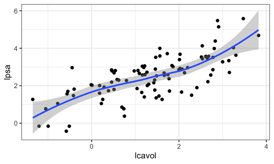
We start off looking at the best one-predictor model, with lcavol predicting lpsa.

ggplot(prostate, aes(x = lcavol, y = lpsa)) + geom_point() + geom_smooth()

## `geom_smooth()` using method = 'loess' and formula = 'y ~ x'

We see that the relationship is pretty close to linear (a line would go through the entire confidence band of the smoother), and so we’re ok with using a linear function of lcavol to predict lpsa.

If there had been a major non-linearity here, we would have wanted to ditch the linear modeling approach and do something non-parametric, maybe loess.

Then we can move to the two-predictor model, and see what the relationship between lcavol, lweight, and lpsa looks like.

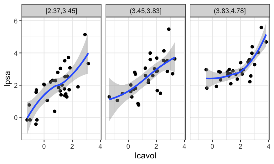
We can make a coplot to examine the relationship between lpsa and lcavol, with lweightas the given variable

ggplot(prostate, aes(x = lcavol, y = lpsa)) + geom_point() + geom_smooth(span = 1) + 
    facet_grid(~cut_number(lweight, n = 3))

## `geom_smooth()` using method = 'loess' and formula = 'y ~ x'

Here it seems like there is some non-linearity, but only for the observations with a high value of lweight.

If we had a lot more observations, this might prompt us to move to loess, but since the non-linearity is based on just a few points, we want to see first whether the non-linearity shows up in other graphs as well.

The best three-predictor model identified by leaps included svi in addition to lcavol and lweight, so we next look at those four variables together.

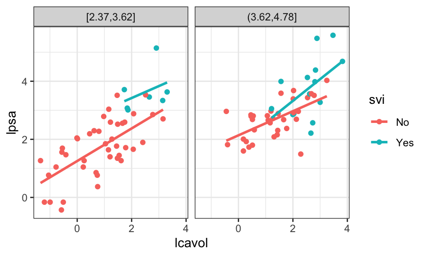
svi is binary and there are only 21 cases where svi is equal to 1, we can’t make a lot of facets and we don’t trust curves that much.

table(prostate$svi)

## 
##  0  1 
## 76 21

prostate$svi = recode(prostate$svi, `1` = "Yes", `0` = "No")
ggplot(prostate, aes(x = lcavol, y = lpsa, group = svi, color = svi)) +
    geom_point() + 
    geom_smooth(method = "lm", se = FALSE) + facet_wrap(~ cut_number(lweight, n = 2))

## `geom_smooth()` using formula = 'y ~ x'

The different slopes suggest an interaction, but again, we don’t have that much data.

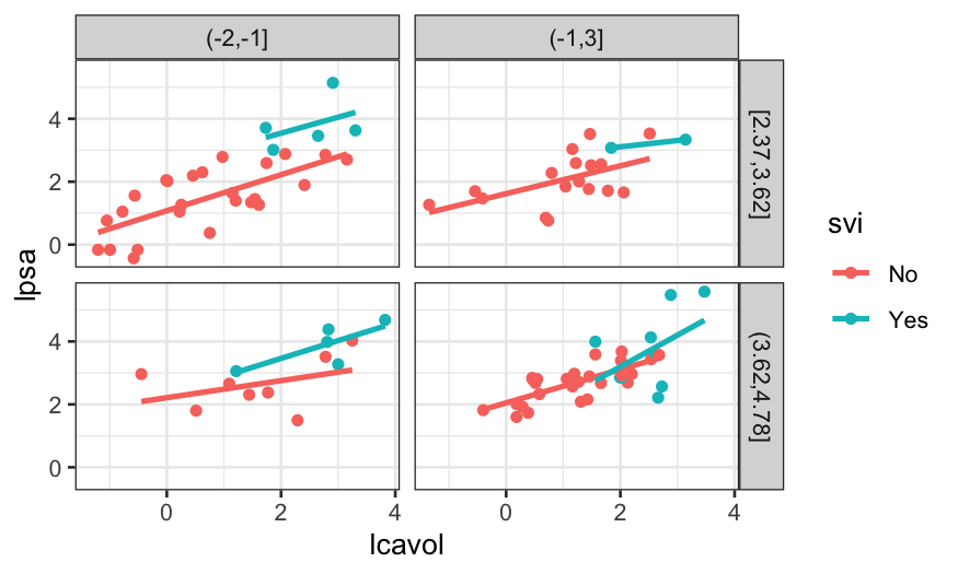
Next we try looking at the predictors from the four-predictor model. This is pushing the limits of the number of variables we can look at all at once, but we will try.

We can look at the relationship between lpsa, lcavol, and svi, with lweight and lbph as the given variables.

ggplot(prostate, aes(x = lcavol, y = lpsa, group = svi, color = svi)) +
    geom_point() + 
    geom_smooth(method = "lm", se = FALSE) +
        facet_grid(cut_number(lweight, n = 2) ~ cut(lbph, breaks = c(-2, -1, 3)))

## `geom_smooth()` using formula = 'y ~ x'

Based on this visualization, we might not be confident about an interaction: the blue lines vary in slope, but there’s based on very small samples. The red lines have different heights but are similar in slope.

Automatic ways of choosing model sizes:

AIC: \(2k - 2 \log(\hat L)\), where \(k\) is the number of parameters in the model and \(\hat L\) is the likelihood at the fitted parameter values.

Mallows’ Cp: Equivalent to AIC for linear regression.

BIC: \(k \log n - 2 \log(\hat L)\), where \(k\) is the number of parameters, \(n\) is the number of observations, and \(\hat L\) is the likelihood at the fitted parameter values.

With each of these, we choose the model with the lowest value of the selection criterion.

In EDA we’re not always required to find a “best” model, and even if we were we can decide on what best means subjectively.

If you wanted to fit a linear model with lcavol, lweight, and svi as predictors plus interactions, you’re free to do so and then call that “best” because of the complexity you can get out of a relatively small number of variables.

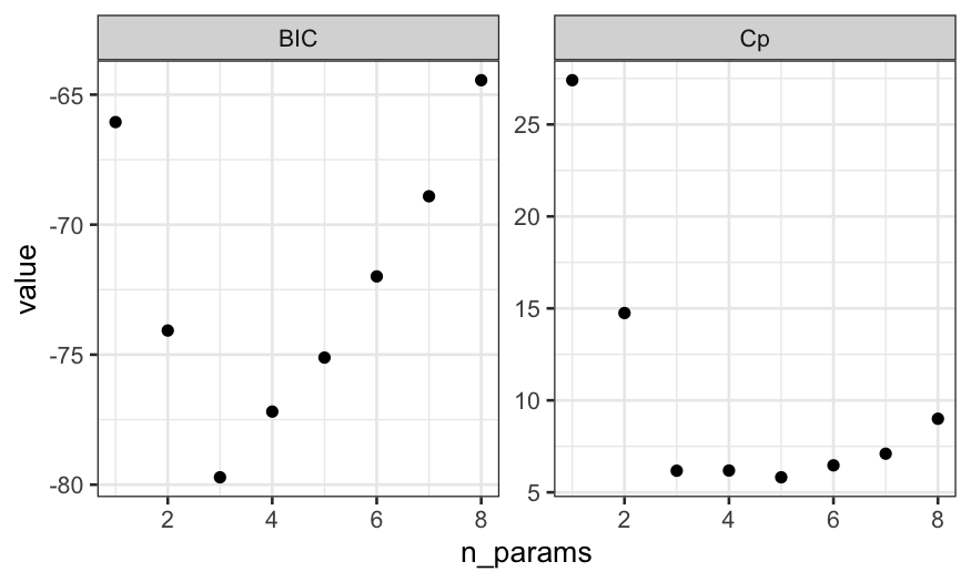
We can also check what the model selection criteria tell us about how many variables to use:

cp_df = data.frame(value  = summary(prostate_best_subset)$cp,
                   n_params = seq_along(summary(prostate_best_subset)$cp),
                   type = "Cp")
bic_df = data.frame(value = summary(prostate_best_subset)$bic,
                    n_params = seq_along(summary(prostate_best_subset)$bic),
                    type = "BIC")
model_selection_criterion_df = rbind(cp_df, bic_df)
ggplot(model_selection_criterion_df, aes(x = n_params, y = value)) +
    geom_point() + facet_wrap(~ type, scales = "free_y")

Even though the lowest value of Cp is for 5 predictors, the Cp value for 3 predictors is very close to the value for 5 predictors and BIC has a strong minimum at 5 predictors. The two plots suggest that if we don’t believe we need any interactions, we should use a model with an intercept and two predictors.

Plotting a final model

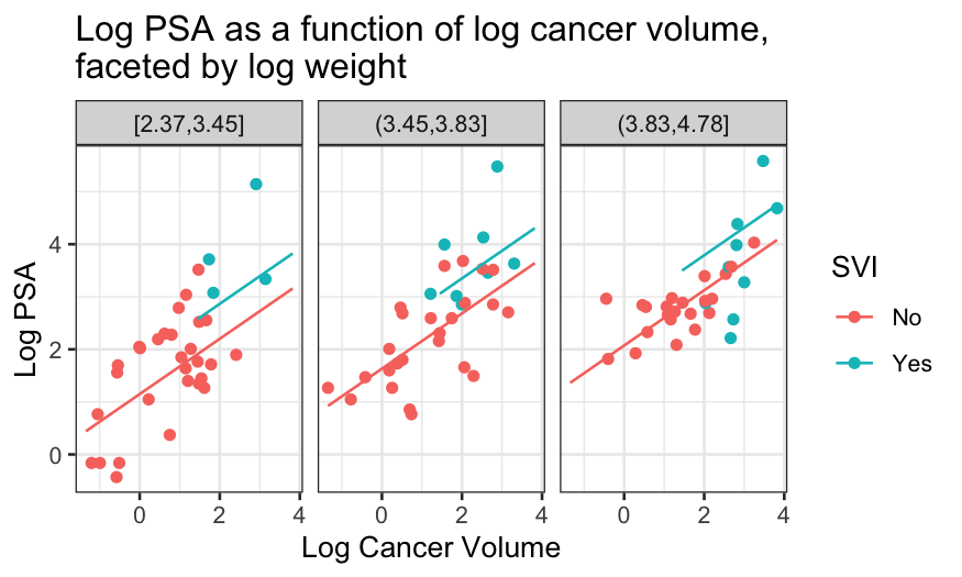
We would like to do a coplot of lpsa as a function of lcavol conditioned on lweight and svi that has fits and predicted values. There are a couple of issues:

Since one of the conditioning variables is continuous, we need to cut that variable up into bins (use cut_number).

We need to get fitted values within each of the bins. Each bin corresponds to a range of values of the conditioning variable lweight, so we need to choose one value to compute a fit at in each of the bins (natural thing to do is use the midpoint of the bin).

The bins are described by a string, not by their midpoint, so we need to compute the midpoint from the string that describes the bins (can use separate and mutate, along with regular expressions).

We will need to merge the information about the fits with the information about the bins (using merge).

lm_final = lm(lpsa ~ lcavol + lweight + svi, data = prostate)
final_fits = augment(lm_final)

## get the bins and the bin means
prostate_with_lweight_bins = prostate %>%
    mutate(lweight_bins = cut_number(lweight, n = 3)) %>%
    separate(lweight_bins, into = c(NA, "lo", "hi", NA), remove = FALSE, sep = "\\[|\\(|\\)|\\]|,") %>%
    mutate(bin_mean = (as.numeric(lo) + as.numeric(hi)) / 2)

## get the grid for prediction
prostate_grid_final = expand.grid(lweight = unique(prostate_with_lweight_bins$bin_mean),
                                  lcavol = quantile(prostate$lcavol),
                                  svi = c("Yes", "No")) %>% data.frame()
## predictions on the grid
prostate_fits_on_grid = augment(lm_final, newdata = prostate_grid_final)
## add information about the bins to the fits
prostate_fits_on_grid = merge(prostate_fits_on_grid,
                             unique(prostate_with_lweight_bins[,c("lweight_bins", "bin_mean")]),
                             by.x = "lweight", by.y = "bin_mean")
## subset so we don't plot the fits outside the range of the data
prostate_fits_on_grid = prostate_fits_on_grid %>% subset(!(svi == "Yes" & lcavol < 1))

ggplot(prostate_with_lweight_bins, aes(x = lcavol, y = lpsa, color = svi)) +
    geom_point() +
    geom_line(aes(y = .fitted), data = prostate_fits_on_grid) +
    facet_wrap(~ lweight_bins) +
    scale_x_continuous("Log Cancer Volume") + scale_y_continuous("Log PSA") +
    scale_color_discrete("SVI") +
    ggtitle("Log PSA as a function of log cancer volume,\nfaceted by log weight")

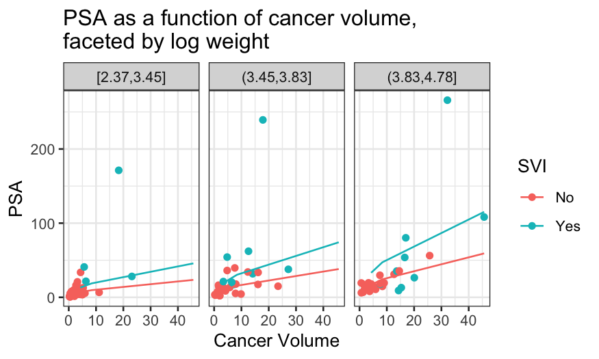
ggplot(prostate_with_lweight_bins, aes(x = exp(lcavol), y = exp(lpsa), color = factor(svi))) +
    geom_point() +
    facet_wrap(~ lweight_bins) +
    geom_line(aes(y = exp(.fitted)), data = prostate_fits_on_grid) +
    scale_x_continuous("Cancer Volume") + scale_y_continuous("PSA") +
    scale_color_discrete("SVI") +
        ggtitle("PSA as a function of cancer volume,\nfaceted by log weight")

Some notes about this model

The final plots highlight some of the deficiencies of the additive model.

Good case to be made for interaction between SVI and log weight.

Looks like at the high values of log weight, there is a non-linear relationship between log PSA and log cancer volume.

Next model to consider might be additive for the low log weights and non-linear with no SVI effect for the high values of log weight.

Overall

There are a couple of automatic ways of choosing the best subsets of predictors and the best model sizes.

These can be used automatically, or they can be used to guide the order in which we investigate whether and how to include variables.

Transformations of the predictors are very important.

Best subsets/forward stepwise/backward stepwise don’t include variables in the same order as the marginal correlations between the predictors and response. Don’t just rely on correlations to decide on which variables to include!