Pairs plot of the three variables
## Registered S3 method overwritten by 'GGally':
##   method from
##   +.gg   ggplot2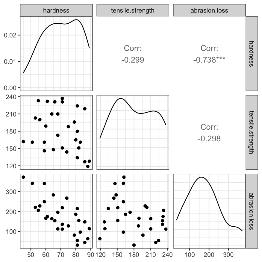
## Registered S3 method overwritten by 'GGally':
## method from
## +.gg ggplot2
coplot_hardness = make_coplot_df(rubber, "hardness", number_bins = 8)
ggplot(coplot_hardness, aes(x = tensile.strength, y = abrasion.loss)) +
    geom_point() +
    facet_wrap(~ interval, ncol = 4) +
    stat_smooth(method = "lm", se = FALSE)
## `geom_smooth()` using formula = 'y ~ x'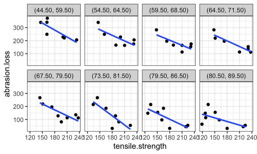
ggplot(coplot_hardness, aes(x = tensile.strength, y = abrasion.loss)) +
    geom_point() +
    facet_wrap(~ interval, ncol = 4) +
    stat_smooth(method = "loess", method.args = list(degree = 1), se = FALSE)
## `geom_smooth()` using formula = 'y ~ x'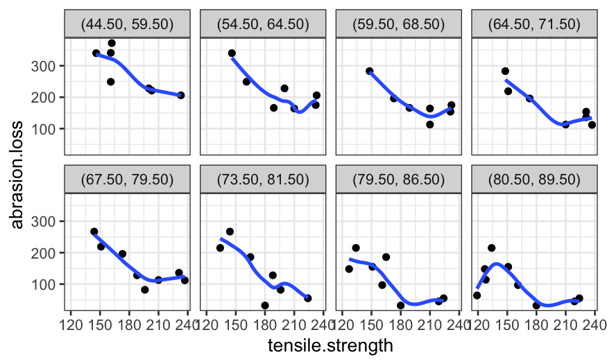
An easier way to make a coplot with ggplot is to use the
cut_number function:
ggplot(rubber, aes(x = tensile.strength, y = abrasion.loss)) +
    geom_point() +
    facet_grid(. ~ cut_number(hardness, n = 4)) +
    stat_smooth(method = "loess", method.args = list(degree = 1, span = .9), se = FALSE)
## `geom_smooth()` using formula = 'y ~ x'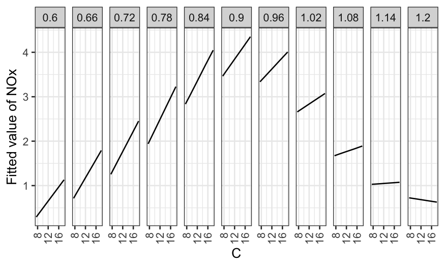
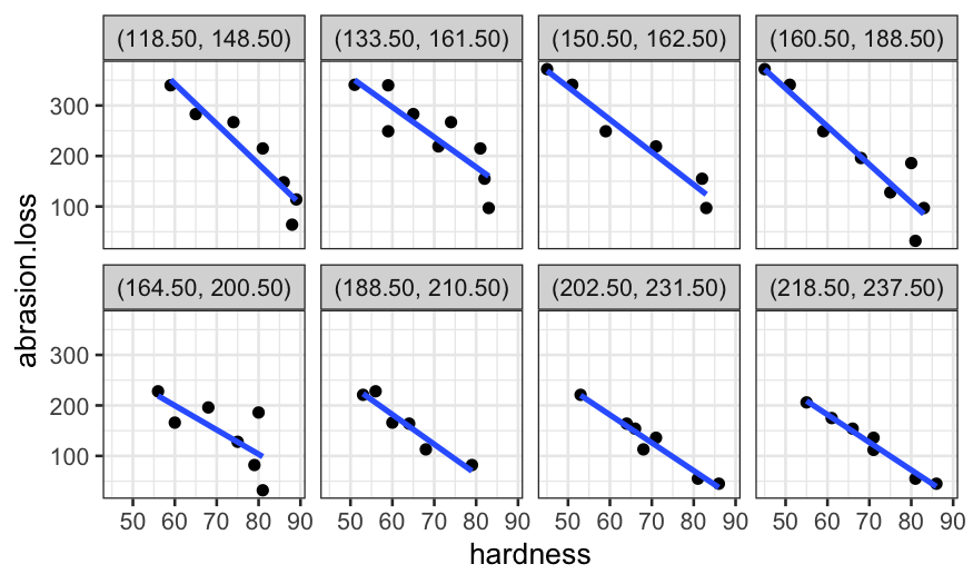
coplot_ts = make_coplot_df(rubber, "tensile.strength", number_bins = 8)
ggplot(coplot_ts, aes(x = hardness, y = abrasion.loss)) +
    geom_point() +
    facet_wrap(~ interval, ncol = 4) +
    stat_smooth(method = "lm", se = FALSE)
## `geom_smooth()` using formula = 'y ~ x'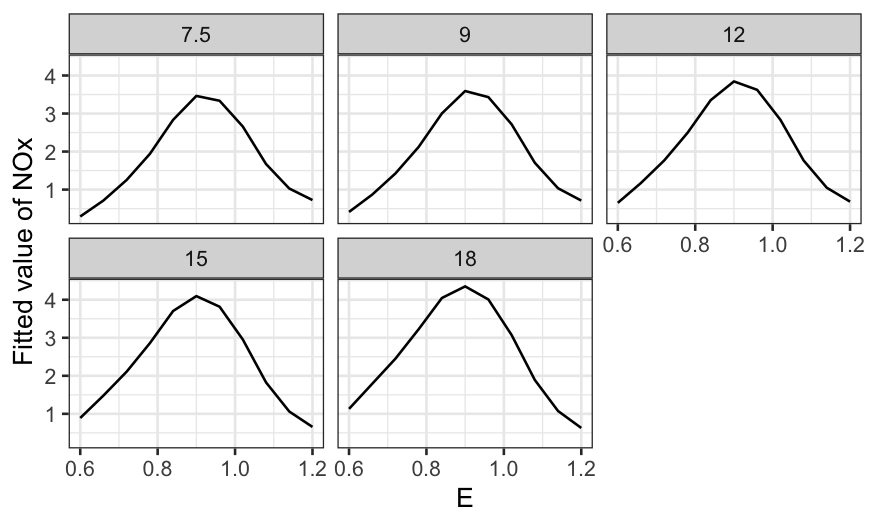
ggplot(coplot_ts, aes(x = hardness, y = abrasion.loss)) +
    geom_point() +
    facet_wrap(~ interval, ncol = 4) +
    stat_smooth(method = "loess", method.args = list(span = .5, degree = 1), se = FALSE)
## `geom_smooth()` using formula = 'y ~ x'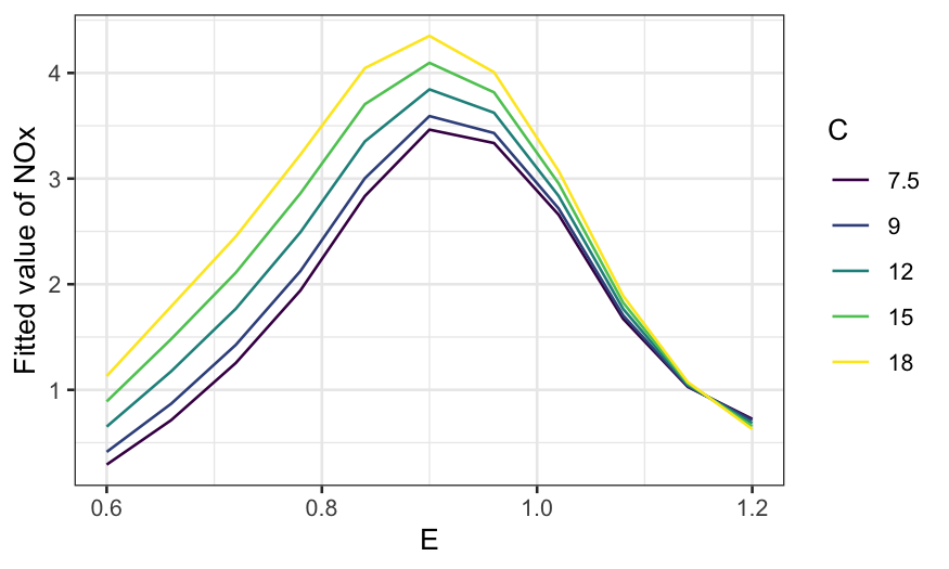
ggplot(coplot_ts, aes(x = hardness, y = abrasion.loss, color = interval)) +
    stat_smooth(method = "loess", method.args = list(span = .5, degree = 1), se = FALSE)
## `geom_smooth()` using formula = 'y ~ x'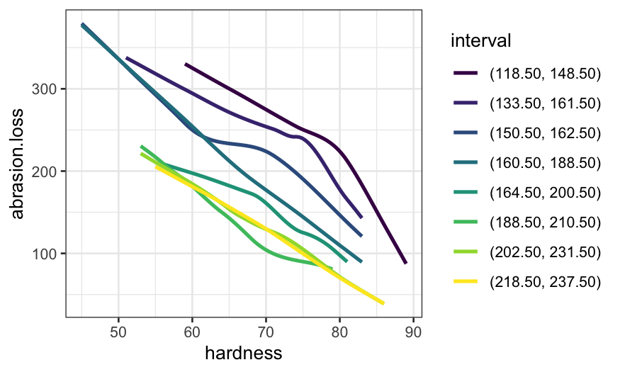
ggplot(coplot_ts, aes(x = hardness, y = abrasion.loss, color = interval)) +
    stat_smooth(method = "lm", se = FALSE)
## `geom_smooth()` using formula = 'y ~ x'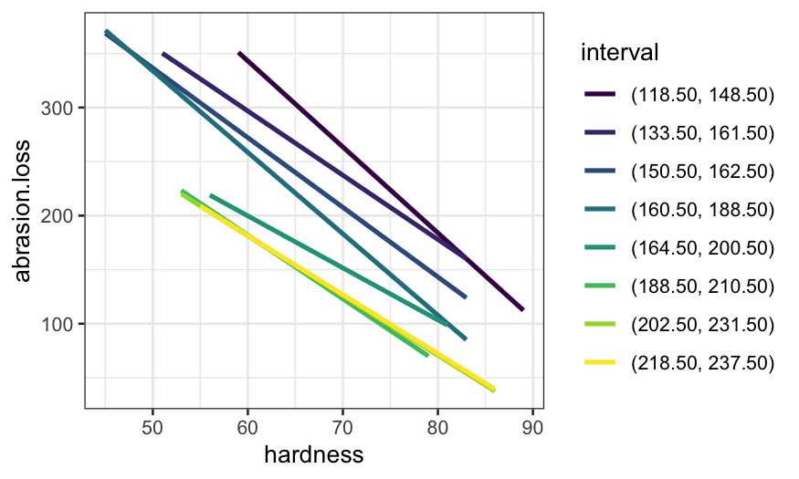
Once we have the fitted values, we can make a coplot of the fitted
model. We’ll start with hardness as the given variable:
ggplot(rubber.predict) +
    geom_line(aes(x = tensile.strength, y = .fitted)) +
    facet_grid(~ hardness) +
    scale_y_continuous("Fitted abrasion loss") +
    theme(axis.text.x = element_text(angle = 90, vjust = 0.5, hjust=1))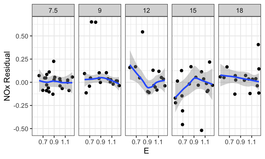
ggplot(rubber.predict) +
    geom_line(aes(x = tensile.strength, y = .fitted, color = factor(hardness, ordered = TRUE))) +
    guides(color = guide_legend(title = "Hardness")) +
    scale_y_continuous("Fitted abrasion loss") +
    theme(axis.text.x = element_text(angle = 90, vjust = 0.5, hjust=1))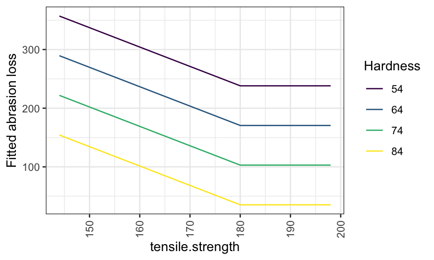
Note that the first plot is a coplot, the second doesn’t have a name but reports the same information in a different way.
Then a coplot with tensile.strength as the given
variable:
ggplot(rubber.predict) +
    geom_line(aes(x = hardness, y = .fitted)) +
    facet_grid(~ tensile.strength) +
    scale_y_continuous("Fitted abrasion loss") +
    theme(axis.text.x = element_text(angle = 90, vjust = 0.5, hjust=1))
ggplot(rubber.predict) +
    geom_line(aes(x = hardness, y = .fitted, color = factor(tensile.strength, ordered = TRUE))) +
    guides(color = guide_legend(title = "Tensile strength")) +
    scale_y_continuous("Fitted abrasion loss") +
    theme(axis.text.x = element_text(angle = 90, vjust = 0.5, hjust=1))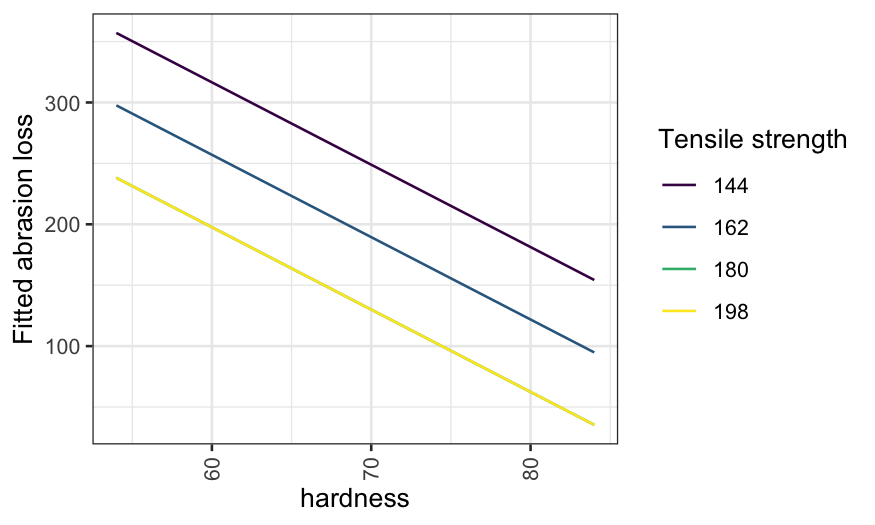
rubber.resid = data.frame(rubber, .resid = residuals(rubber.rlm))
ggplot(rubber.resid, aes(x = tensile.strength, y = .resid)) + geom_point() +
    stat_smooth(method = "loess", span = 1, method.args = list(degree = 1, family = "symmetric")) +
    geom_abline(slope = 0, intercept = 0) +
    scale_y_continuous("Abrasion loss residuals")
## `geom_smooth()` using formula = 'y ~ x'
ggplot(rubber.resid, aes(x = hardness, y = .resid)) + geom_point() +
    stat_smooth(method = "loess", span = 1, method.args = list(degree = 1, family = "symmetric")) +
    geom_abline(slope = 0, intercept = 0) +
    scale_y_continuous("Abrasion loss residuals")
## `geom_smooth()` using formula = 'y ~ x'
resid_co_hardness = make_coplot_df(rubber.resid, faceting_variable = "hardness", number_bins = 4)
ggplot(resid_co_hardness, aes(x = tensile.strength, y = .resid)) +
    geom_point() +
    facet_grid(~ interval) +
    stat_smooth(method = "loess", method.args = list(degree = 1, family = "symmetric")) +
    scale_y_continuous("Abrasion loss residuals")
## `geom_smooth()` using formula = 'y ~ x'
resid_co_ts = make_coplot_df(rubber.resid, faceting_variable = "tensile.strength", number_bins = 4)
ggplot(resid_co_ts, aes(x = hardness, y = .resid)) +
    geom_point() +
    facet_grid(~ interval) +
    stat_smooth(method = "loess", method.args = list(degree = 1, family = "symmetric")) +
    scale_y_continuous("Abrasion loss residuals")
## `geom_smooth()` using formula = 'y ~ x'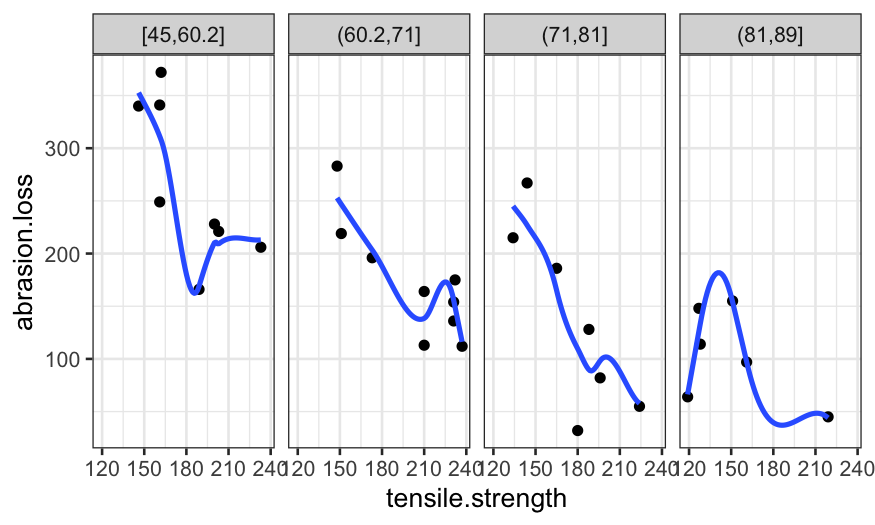
From the residual plots, it looks like we might actually do better
fitting an interaction between tensile.strength and
hardness.
Below, we fit a model with the interaction and make a coplot of the fitted and actual values.
We see that with the interaction, the slope of the fit below tensile strengh of 180 changes with hardness (steepest for the lowest values of hardness, shallowest for the highest hardnesses).
rubber.rlm = rlm(abrasion.loss ~ hardness * ts.low, data = rubber, psi = psi.bisquare)
coplot_hardness = coplot_hardness %>% mutate(interval_mean = get_interval_means(interval))
rubber.grid.final = expand.grid(hardness = unique(coplot_hardness$interval_mean),
                          tensile.strength = c(125, 180, 240)) %>% data.frame
rubber.grid.final = rubber.grid.final |> mutate(ts.low = tslow(tensile.strength))
rubber.predict.final = augment(rubber.rlm, newdata = rubber.grid.final)
rubber.predict.final = merge(rubber.predict.final,
                             unique(coplot_hardness[,c("interval", "interval_mean")]),
                             by.x = "hardness", by.y = "interval_mean")

ggplot(coplot_hardness, aes(x = tensile.strength, y = abrasion.loss)) +
    geom_point() +
    geom_line(aes(x = tensile.strength, y = .fitted), data = rubber.predict.final) +
    facet_wrap(~ interval, ncol = 4) +
    scale_y_continuous("Abrasion loss") +
    scale_x_continuous("Tensile strength")