The Bayesian Goal

In Bayesian inference, we want to compute the posterior distribution over the parameters: \[ P(\theta \mid x_1,\ldots, x_n) = \frac{P(x_1, \ldots, x_n \mid \theta)P(\theta)}{P(x_1,\ldots, x_n)} \]

Notes:

Sometimes there is an analytic solution.
If there is no analytic solution, we try to sample from \(P(\theta \mid x_1,\ldots, x_n)\) instead.
Most of the time it is hard to compute \(P(x_1, \ldots, x_n)\).
To use Metropolis-Hastings to sample from \(P(\theta \mid x_1,\ldots, x_n)\), we only need to be able to compute \(P(x_1, \ldots, x_n \mid \theta)P(\theta)\).

Example 1: Estimating a correlation

(Example 5.2 in the book). We have two variables measured on \(n\) cases, and we would like to estimate the correlation between them.

For this problem, we have

Data: \(x_i \in \mathbb R^2\), \(i = 1,\ldots, n\)
Model: \[ P(x_i \mid \mu_1, \mu_2, \sigma_1, \sigma_2, r) = \mathcal N_2 \left( \begin{pmatrix}\mu_1 \\ \mu_2 \end{pmatrix}, \begin{pmatrix} \sigma_1^2 & r \sigma_1 \sigma_2 \\ r \sigma_1 \sigma_2 & \sigma_2^2 \end{pmatrix} \right) \]
Parameters: \(\mu_1, \mu_2, \sigma_1, \sigma_2, r\)
Prior on the parameters: \[ \begin{align*} P(\mu_1) &= \mathcal N(0, 1000)\\ P(\mu_2) &= \mathcal N(0, 1000)\\ P(\sigma_1) &= \text{InvSqrtGamma}(.001, .001)\\ P(\sigma_2) &= \text{InvSqrtGamma}(.001, .001)\\ P(r) &= \text{Uniform}(-1,1) \end{align*} \]

Posterior distribution on the parameters: \[ P(\mu_1, \mu_2,\sigma_1, \sigma_2, r \mid x_1, \ldots, x_n) \propto \prod_{i=1}^n P(x_i \mid \mu_1, \mu_2, \sigma_1, \sigma_2, r) P(\mu_1) P(\mu_2) P(\sigma_1) P(\sigma_2) P(r) \]

Everything on the right-hand side is easily computable, and that is all we need for MCMC.

What would Metropolis-Hastings look like here?

Start with some initial values of the parameters: \(\mu_1^{(0)}, \mu_2^{(0)}, \sigma_1^{(0)}, \sigma_2^{(0)}, r^{(0)}\)

For i in 1 to as many iterations as desired:

Propose a new set of parameters \(\mu_1^{(i)}, \mu_2^{(i)}, \sigma_1^{(i)}, \sigma_2^{(i)}, r^{(i)}\) from a proposal distribution around \(\mu_1^{(i-1)}, \mu_2^{(i-1)}, \sigma_1^{(i-1)}, \sigma_2^{(i-1)}, r^{(i-1)}\).
Compute the ratio \[ \begin{align*} a = &\frac{P(\mu_1^{(i)}, \mu_2^{(i)}, \sigma_1^{(i)}, \sigma_2^{(i)}, r^{(i)} \mid x_1,\ldots, x_n)}{P(\mu_1^{(i)}, \mu_2^{(i)}, \sigma_1^{(i)}, \sigma_2^{(i)}, r^{(i)} \mid x_1,\ldots, x_n )} \\ \quad &= \frac{ \prod_{i=1}^n P(x_i \mid \mu_1^{(i)}, \mu_2^{(i)}, \sigma_1^{(i)}, \sigma_2^{(i)}, r^{(i)}) P(\mu_1^{(i)}) P(\mu_2^{(i)}) P(\sigma_1^{(i)}) P(\sigma_2^{(i)}) P(r^{(i)})}{ \prod_{i=1}^n P(x_i \mid \mu_1^{(i-1)}, \mu_2^{(i-1)}, \sigma_1^{(i-1)}, \sigma_2^{(i-1)}, r^{(i-1)}) P(\mu_1^{(i-1)}) P(\mu_2^{(i-1)}) P(\sigma_1^{(i-1)}) P(\sigma_2^{(i-1)}) P(r^{(i-1)})} \end{align*} \]
If \(a > 1\), move to the proposed set of parameters, otherwise move to the proposed set of parameters with probability \(a\) and stay at the current set with probability \(1 - a\)

model_correlation <- "
// Pearson Correlation
data { 
  int<lower=0> n;
  vector[2] x[n];
}
parameters {
  vector[2] mu;
  vector<lower=0>[2] lambda;
  real<lower=-1,upper=1> r;
} 
transformed parameters {
  vector<lower=0>[2] sigma;
  cov_matrix[2] T;
  // Reparameterization
  sigma[1] = inv_sqrt(lambda[1]);
  sigma[2] = inv_sqrt(lambda[2]);
  T[1,1] = square(sigma[1]);
  T[1,2] = r * sigma[1] * sigma[2];
  T[2,1] = r * sigma[1] * sigma[2];
  T[2,2] = square(sigma[2]);
}
model {
  // Priors
  mu ~ normal(0, inv_sqrt(.001));
  lambda ~ gamma(.001, .001);
  
  // Data
  x ~ multi_normal(mu, T);
}"

# The dataset:
  x <- matrix(c( .8, 102, 
                1.0,  98, 
                 .5, 100,
                 .9, 105, 
                 .7, 103, 
                 .4, 110,
                1.2,  99, 
                1.4,  87,
                 .6, 113,
                1.1,  89,
                1.3,  93), nrow=11, ncol=2, byrow=T) 

n <- nrow(x) # number of people/units measured

data <- list(x=x, n=n) # to be passed on to Stan
myinits <- list(
  list(r=0, mu=c(0, 0), lambda=c(1, 1)))

# parameters to be monitored: 
parameters <- c("r", "mu", "sigma")

samples <- stan(model_code=model_correlation,   
                data=data, 
                init=myinits,
                pars=parameters,
                iter=10000, 
                chains=1, 
                thin=1)

## 
## SAMPLING FOR MODEL '31aefbc6f9701279b306e349956c379c' NOW (CHAIN 1).
## Chain 1: 
## Chain 1: Gradient evaluation took 8.8e-05 seconds
## Chain 1: 1000 transitions using 10 leapfrog steps per transition would take 0.88 seconds.
## Chain 1: Adjust your expectations accordingly!
## Chain 1: 
## Chain 1: 
## Chain 1: Iteration:    1 / 10000 [  0%]  (Warmup)
## Chain 1: Iteration: 1000 / 10000 [ 10%]  (Warmup)
## Chain 1: Iteration: 2000 / 10000 [ 20%]  (Warmup)
## Chain 1: Iteration: 3000 / 10000 [ 30%]  (Warmup)
## Chain 1: Iteration: 4000 / 10000 [ 40%]  (Warmup)
## Chain 1: Iteration: 5000 / 10000 [ 50%]  (Warmup)
## Chain 1: Iteration: 5001 / 10000 [ 50%]  (Sampling)
## Chain 1: Iteration: 6000 / 10000 [ 60%]  (Sampling)
## Chain 1: Iteration: 7000 / 10000 [ 70%]  (Sampling)
## Chain 1: Iteration: 8000 / 10000 [ 80%]  (Sampling)
## Chain 1: Iteration: 9000 / 10000 [ 90%]  (Sampling)
## Chain 1: Iteration: 10000 / 10000 [100%]  (Sampling)
## Chain 1: 
## Chain 1:  Elapsed Time: 1.29576 seconds (Warm-up)
## Chain 1:                1.18674 seconds (Sampling)
## Chain 1:                2.4825 seconds (Total)
## Chain 1:

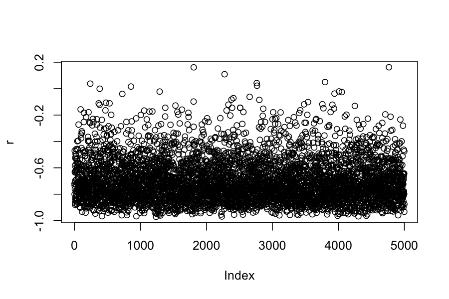
r <- extract(samples)$r
plot(r)

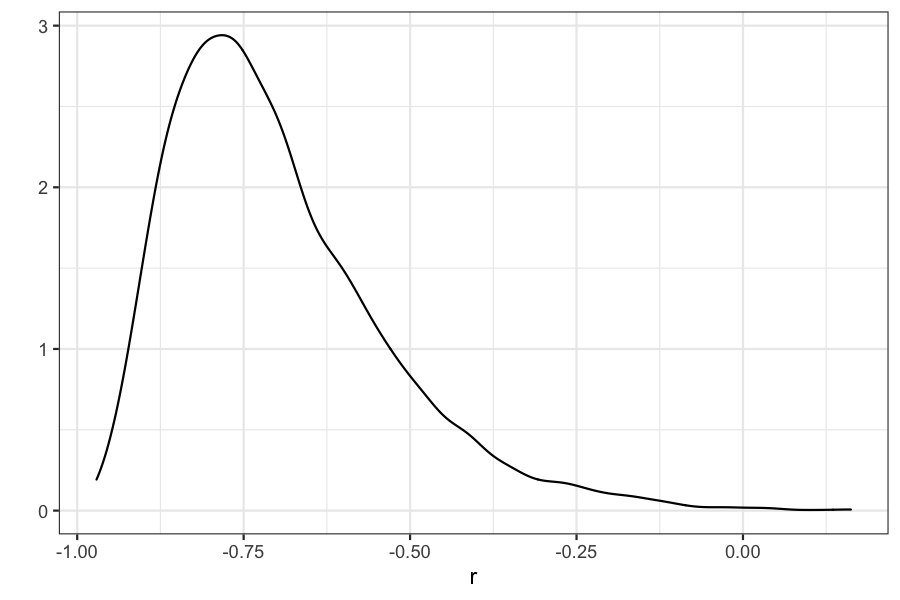
qplot(r, geom = "density")

## 95% credible interval
quantile(r, c(.025, .975))

##       2.5%      97.5% 
## -0.9195804 -0.2890643

## posterior mean
mean(r)

## [1] -0.6997152

#Frequentist point-estimate of r:
(freq.r <- cor(x[,1],x[,2]))

## [1] -0.8109671

Estimating a correlation with measurement error

(Example 5.2 in the book)

Problem: Suppose that our data come from a study of the relationship between “response time on a semantic verification task” and IQ.

The researchers want to estimate the correlation between response time and IQ.
The problem is that the IQ measurement has some uncertainty associated with it, and so the previous model we used to estimate the correlation is incorrect.

For the model with uncertainy in measurements, we again have two variables (response time and IQ) measured on \(n\) cases, and we would like to estimate the correlation between them.

Data: \(x_i \in \mathbb R^2\), \(i = 1,\ldots, n\)
Model: \[ \begin{align*} P(y_i \mid \mu_1, \mu_2, \sigma_1, \sigma_2, r) &= \mathcal N_2 \left( \begin{pmatrix}\mu_1 \\ \mu_2 \end{pmatrix}, \begin{pmatrix} \sigma_1^2 & r \sigma_1 \sigma_2 \\ r \sigma_1 \sigma_2 & \sigma_2^2 \end{pmatrix} \right)\\ P(x_{i} \mid y_{i}) &= \mathcal N_2\left(y_{i}, \begin{pmatrix} \sigma^e_1 & 0 \\ 0 & \sigma_2^e \end{pmatrix} \right) \end{align*} \]
Parameters: \(\mu_1, \mu_2, \sigma_1, \sigma_2, r\) (we assume that the measurement errors, \(\sigma^e_1, \sigma^e_2\), are known)
Prior on the parameters: \[ \begin{align*} P(\mu_1) &= \mathcal N(0, 1000)\\ P(\mu_2) &= \mathcal N(0, 1000)\\ P(\sigma_1) &= \text{InvSqrtGamma}(.001, .001)\\ P(\sigma_2) &= \text{InvSqrtGamma}(.001, .001)\\ P(r) &= \text{Uniform}(-1,1) \end{align*} \]

Posterior distribution:

\[ P( \mu_1, \mu_2, \sigma_1, \sigma_2, r \mid x_1,\ldots, x_n) \propto \prod_{i=1}^n P(x_i \mid y_i) P(y_i \mid \mu_1, \mu_2, \sigma_1, \sigma_2, r) P(\mu_1)P(\mu_2)P(\sigma_1)P(\sigma_2)P(r) \]

Again, everything is easily computable, and we can use MCMC to obtain samples from the posterior distribution.

model <- "
// Pearson Correlation With Uncertainty in Measurement
data { 
  int<lower=0> n;
  vector[2] x[n];
  vector[2] sigmaerror;
}
parameters {
  vector[2] mu;
  vector<lower=0>[2] lambda;
  real<lower=-1,upper=1> r;
  vector[2] y[n];
} 
transformed parameters {
  vector<lower=0>[2] sigma;
  cov_matrix[2] T;
  // Reparameterization
  sigma[1] = inv_sqrt(lambda[1]);
  sigma[2] = inv_sqrt(lambda[2]);
  
  T[1,1] = square(sigma[1]);
  T[1,2] = r * sigma[1] * sigma[2];
  T[2,1] = r * sigma[1] * sigma[2];
  T[2,2] = square(sigma[2]);
}
model {
  // Priors
  mu ~ normal(0, inv_sqrt(.001));
  lambda ~ gamma(.001, .001);
  // Data
  y ~ multi_normal(mu, T);
  for (i in 1:n)
    x[i] ~ normal(y[i], sigmaerror);
}"

x <- matrix(c( .8, 102, 
              1.0,  98, 
               .5, 100,
               .9, 105, 
               .7, 103, 
               .4, 110,
              1.2,  99, 
              1.4,  87,
               .6, 113,
              1.1,  89,
              1.3,  93), nrow=11, ncol=2, byrow=T) 

n <- nrow(x) # number of people/units measured

# precision of measurement:
sigmaerror <- c(.03, 5)

data <- list(x=x, n=n, sigmaerror=sigmaerror) # to be passed on to Stan
myinits <- list(
  list(r=0, mu=c(0, 0), lambda=c(1, 1), y=matrix(c(rep(1, n), rep(100, n)), n, 2)))

# parameters to be monitored:  
parameters <- c("r", "mu", "sigma")
samples <- stan(model_code=model,   
                data=data, 
                init=myinits,
                pars=parameters,
                iter=20000, 
                chains=1, 
                thin=1,
                algorithm="HMC")

## 
## SAMPLING FOR MODEL 'ca98a184003e9d2907fcd31a07a7d500' NOW (CHAIN 1).
## Chain 1: 
## Chain 1: Gradient evaluation took 7.7e-05 seconds
## Chain 1: 1000 transitions using 10 leapfrog steps per transition would take 0.77 seconds.
## Chain 1: Adjust your expectations accordingly!
## Chain 1: 
## Chain 1: 
## Chain 1: Iteration:     1 / 20000 [  0%]  (Warmup)
## Chain 1: Iteration:  2000 / 20000 [ 10%]  (Warmup)
## Chain 1: Iteration:  4000 / 20000 [ 20%]  (Warmup)
## Chain 1: Iteration:  6000 / 20000 [ 30%]  (Warmup)
## Chain 1: Iteration:  8000 / 20000 [ 40%]  (Warmup)
## Chain 1: Iteration: 10000 / 20000 [ 50%]  (Warmup)
## Chain 1: Iteration: 10001 / 20000 [ 50%]  (Sampling)
## Chain 1: Iteration: 12000 / 20000 [ 60%]  (Sampling)
## Chain 1: Iteration: 14000 / 20000 [ 70%]  (Sampling)
## Chain 1: Iteration: 16000 / 20000 [ 80%]  (Sampling)
## Chain 1: Iteration: 18000 / 20000 [ 90%]  (Sampling)
## Chain 1: Iteration: 20000 / 20000 [100%]  (Sampling)
## Chain 1: 
## Chain 1:  Elapsed Time: 14.3309 seconds (Warm-up)
## Chain 1:                11.029 seconds (Sampling)
## Chain 1:                25.3599 seconds (Total)
## Chain 1:

r <- extract(samples)$r
plot(r)

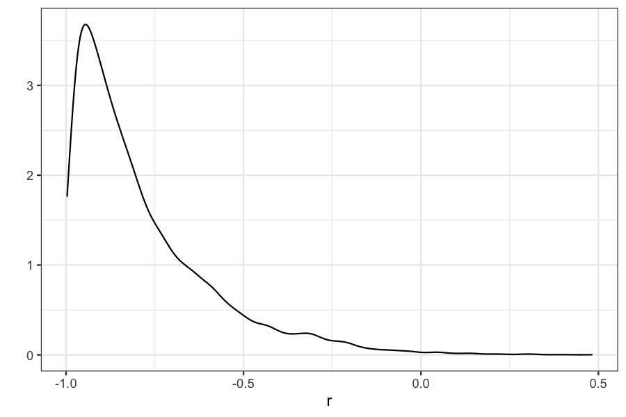
## posterior density for r
qplot(r, geom = "density")

## 95% credible interval
quantile(r, c(.025, .975))

##       2.5%      97.5% 
## -0.9884777 -0.2521108

## posterior mean
mean(r)

## [1] -0.7856381

#Frequentist point-estimate of r:
(freq.r <- cor(x[,1],x[,2]))

## [1] -0.8109671

Example 3: Seven scientists

(Example 4.2 in the book). Seven scientists with dramatically different capabilities run an experiment to measure a certain quantity.

The get the results: -27.020, 3.570, 8.191, 9.898, 9.603, 9.945, 10.056

We would like to combine their results to get an estimate of the true value of the quantity they were trying to measure.

We can model this as:

The result each of the scientists obtained comes from a normal distribution
All seven distributions have the same mean
All seven distributions have different variances

Listing everything out:

Data: \(x_i \in \mathbb R^1\), \(i = 1,\ldots, 7\)
Likelihood: \[ P(x_i \mid \mu, \lambda_i ) = \mathcal N(\mu, \lambda_i^{-1}) \]
Parameters: \(\mu, \lambda_1,\ldots, \lambda_7\)
Prior: \[ \begin{align*} P(\mu) &= \mathcal N(0, 1000) \\ P(\lambda_i) &= \text{Gamma}(.001, .001) \end{align*} \]

Posterior: \[ P(\mu, \lambda_1,\ldots, \lambda_7 \mid x_1,\ldots, x_7) \propto \prod_{i=1}^7 P(x_i \mid \mu, \lambda_1,\ldots, \lambda_7) P(\mu) \prod_{i=1}^7 P(\lambda_i) \]

Again, everything on the right can be evaluated easily, and we can use MCMC to sample from the distribution.

model_seven_scientists = "
// The Seven Scientists
data { 
  int<lower=1> n;
  vector[n] x;
}
parameters {
  real mu;
  vector<lower=0>[n] lambda;
} 
transformed parameters {
  vector[n] sigma;
  
  for (i in 1:n)
    sigma[i] = inv_sqrt(lambda[i]);
}
model {
  // Priors
  mu ~ normal(0, sqrt(1000));
  lambda ~ gamma(.001, .001);
  
  // Data Come From Gaussians With Common Mean But Different Precisions
  x ~ normal(mu, sigma);
}"

x <- c(-27.020, 3.570, 8.191, 9.898, 9.603, 9.945, 10.056)
n <- length(x)

data <- list(x=x, n=n) # to be passed on to Stan
myinits <- list(
  list(mu=0, lambda=rep(1,n)))

# parameters to be monitored:  
parameters <- c("mu", "lambda")

samples_seven_scientists <- stan(model_code=model_seven_scientists,   
                data=data, 
                init=myinits,
                pars=parameters,
                iter=20000, 
                chains=1, 
                thin=1,
                algorithm="HMC")

## 
## SAMPLING FOR MODEL '0ad4c94821220e5bc1c79495c2929f20' NOW (CHAIN 1).
## Chain 1: 
## Chain 1: Gradient evaluation took 2.1e-05 seconds
## Chain 1: 1000 transitions using 10 leapfrog steps per transition would take 0.21 seconds.
## Chain 1: Adjust your expectations accordingly!
## Chain 1: 
## Chain 1: 
## Chain 1: Iteration:     1 / 20000 [  0%]  (Warmup)
## Chain 1: Iteration:  2000 / 20000 [ 10%]  (Warmup)
## Chain 1: Iteration:  4000 / 20000 [ 20%]  (Warmup)
## Chain 1: Iteration:  6000 / 20000 [ 30%]  (Warmup)
## Chain 1: Iteration:  8000 / 20000 [ 40%]  (Warmup)
## Chain 1: Iteration: 10000 / 20000 [ 50%]  (Warmup)
## Chain 1: Iteration: 10001 / 20000 [ 50%]  (Sampling)
## Chain 1: Iteration: 12000 / 20000 [ 60%]  (Sampling)
## Chain 1: Iteration: 14000 / 20000 [ 70%]  (Sampling)
## Chain 1: Iteration: 16000 / 20000 [ 80%]  (Sampling)
## Chain 1: Iteration: 18000 / 20000 [ 90%]  (Sampling)
## Chain 1: Iteration: 20000 / 20000 [100%]  (Sampling)
## Chain 1: 
## Chain 1:  Elapsed Time: 1.12893 seconds (Warm-up)
## Chain 1:                1.73411 seconds (Sampling)
## Chain 1:                2.86305 seconds (Total)
## Chain 1:

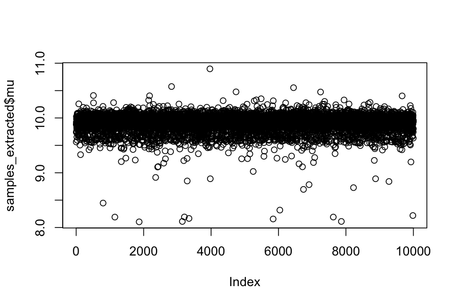
samples_extracted <- extract(samples_seven_scientists)
## show the chain
plot(samples_extracted$mu)

## posterior mean of mu
mean(samples_extracted$mu)

## [1] 9.908714

## frequentist mean of mu
mean(x)

## [1] 3.463286

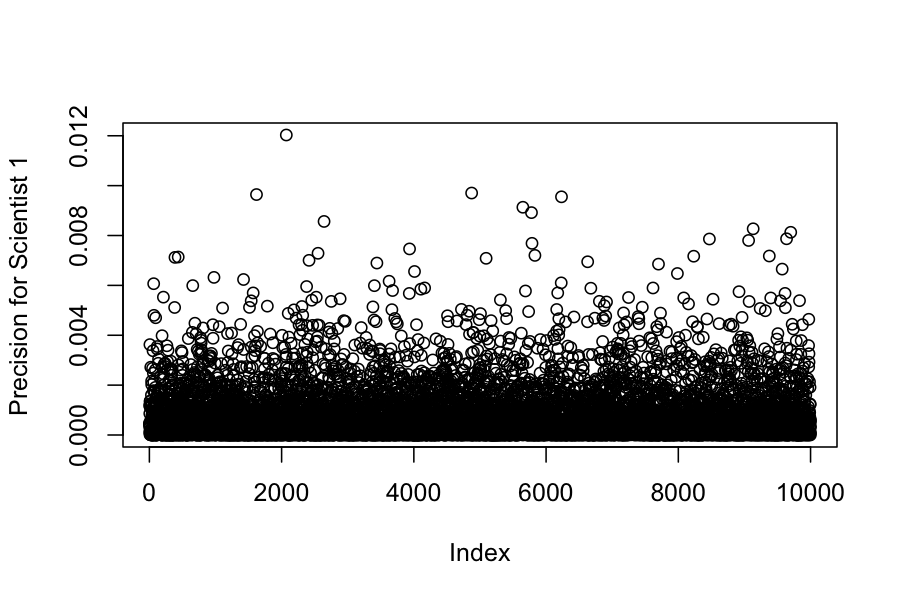
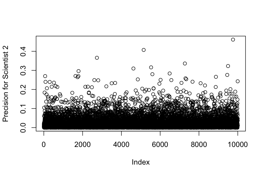
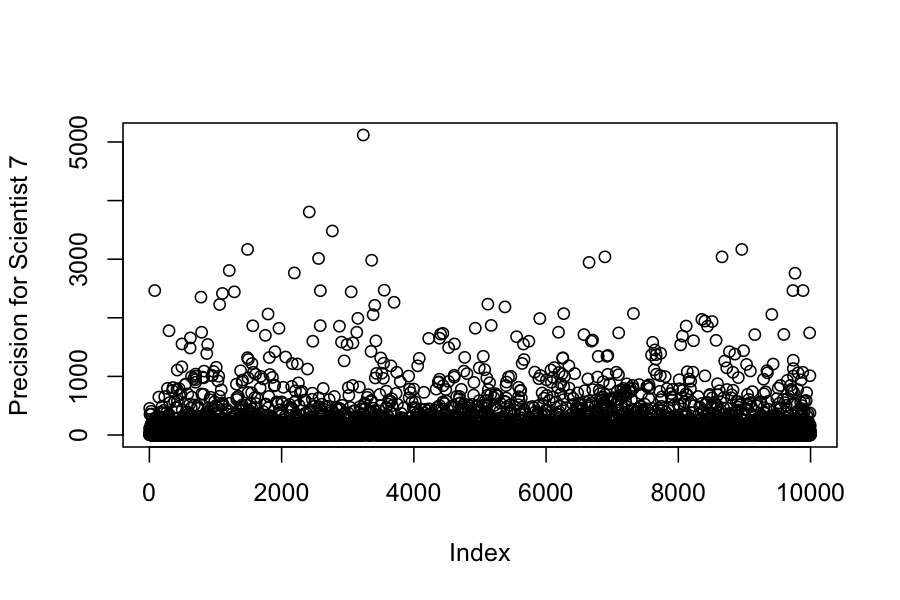
We can also look at the posteriors for each of the variances:

plot(samples_extracted$lambda[,1], ylab = "Precision for Scientist 1")

plot(samples_extracted$lambda[,2], ylab = "Precision for Scientist 2")

plot(samples_extracted$lambda[,7], ylab = "Precision for Scientist 7")

round(apply(samples_extracted$lambda, 2, mean), digits = 4)

## [1]   0.0007   0.0251   0.5750 209.2929  31.2783 223.3959 105.5578

Example 4: Changepoint detection

(Example 5.4 in the book)

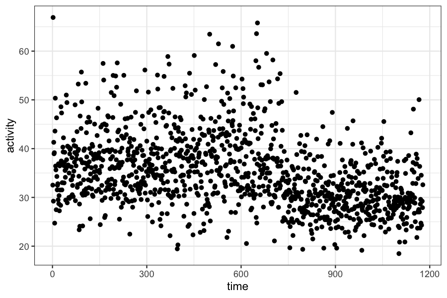
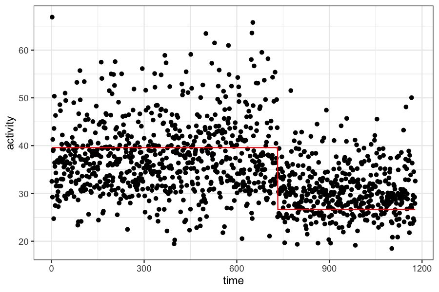
We have data on frontal lobe activity in a study of adults with ADHD.

In the experiment, we expect to see a “changepoint” in the measure of frontal lobe activity. The mean activity level will be different before and after the changepoint, and we want to estimate both the time of the change and the mean activity level before and after.

c <- scan("changepointdata.txt")
ggplot(data.frame(activity = c, time = 1:length(c))) + geom_point(aes(x = time, y = activity))

Listing everything out:

Data: \(x_i \in \mathbb R\), \(i = 1,\ldots, n\)
Likelihood: \[ P(x_i \mid \mu_1, \mu_2, \tau, \lambda ) = \begin{cases} \mathcal N(\mu_1, \lambda^{-1}) & i \le \tau \\ \mathcal N(\mu_2, \lambda^{-1}) & i > \tau \end{cases} \]
Parameters: \(\mu_1, \mu_2, \tau, \lambda\)
Prior: \[ \begin{align*} P(\mu_1) &= \mathcal N(0, 1000) \\ P(\mu_2) &= \mathcal N(0, 1000) \\ P(\lambda) &= \text{Gamma}(.001, .001)\\ P(\tau) &= \text{Uniform}(0, n) \end{align*} \]

Posterior: \[ P(\mu_1, \mu_2, \lambda, \tau \mid x_1,\ldots, x_n) \propto \prod_{i=1}^n P(x_i \mid \mu_1, \mu_2 \lambda, \tau) P(\mu_1) P(\mu_2) P(\lambda) P(\tau) \]

Again, everything on the right can be evaluated easily, and we can use MCMC to sample from the distribution.

model_changepoint <- "
// Change Detection
data { 
  int n;
  vector[n] t;
  vector[n] c;
}
parameters {
  vector[2] mu;
  real<lower=0> lambda;
  real<lower=0,upper=n> tau;
} 
transformed parameters {
  real<lower=0> sigma;
  sigma = inv_sqrt(lambda);
}
model { 
  // Group Means
  mu ~ normal(0, inv_sqrt(.001));
  // Common Precision
  lambda ~ gamma(.001, .001);
    
  // Which Side is Time of Change Point?
  // Data Come From A Gaussian
  for (i in 1:n) {
    if ((t[i] - tau) < 0.0)
      c[i] ~ normal(mu[1], sigma);
    else 
      c[i] ~ normal(mu[2], sigma);
  }
}"

c <- scan("changepointdata.txt")
n <- length(c)
t <- 1:n

data <- list(c=c, n=n, t=t) # to be passed on to Stan
myinits <- list(
  list(mu=c(1, 1), lambda=1, tau=n / 2))

# parameters to be monitored:  
parameters <- c("mu", "sigma", "tau")

samples_changepoint <- stan(model_code=model_changepoint,   
                data=data, 
                init=myinits,
                pars=parameters,
                iter=250, 
                chains=1, 
                thin=1,
                warmup = 150,
                seed = 1,
                control=list(max_treedepth=12))

## 
## SAMPLING FOR MODEL 'e72b21df214cd793eaea2913a67de562' NOW (CHAIN 1).
## Chain 1: 
## Chain 1: Gradient evaluation took 8.6e-05 seconds
## Chain 1: 1000 transitions using 10 leapfrog steps per transition would take 0.86 seconds.
## Chain 1: Adjust your expectations accordingly!
## Chain 1: 
## Chain 1: 
## Chain 1: Iteration:   1 / 250 [  0%]  (Warmup)
## Chain 1: Iteration:  25 / 250 [ 10%]  (Warmup)
## Chain 1: Iteration:  50 / 250 [ 20%]  (Warmup)
## Chain 1: Iteration:  75 / 250 [ 30%]  (Warmup)
## Chain 1: Iteration: 100 / 250 [ 40%]  (Warmup)
## Chain 1: Iteration: 125 / 250 [ 50%]  (Warmup)
## Chain 1: Iteration: 150 / 250 [ 60%]  (Warmup)
## Chain 1: Iteration: 151 / 250 [ 60%]  (Sampling)
## Chain 1: Iteration: 175 / 250 [ 70%]  (Sampling)
## Chain 1: Iteration: 200 / 250 [ 80%]  (Sampling)
## Chain 1: Iteration: 225 / 250 [ 90%]  (Sampling)
## Chain 1: Iteration: 250 / 250 [100%]  (Sampling)
## Chain 1: 
## Chain 1:  Elapsed Time: 30.4862 seconds (Warm-up)
## Chain 1:                23.8348 seconds (Sampling)
## Chain 1:                54.321 seconds (Total)
## Chain 1:

# Now the values for the monitored parameters are in the "samples" object, 
# ready for inspection.
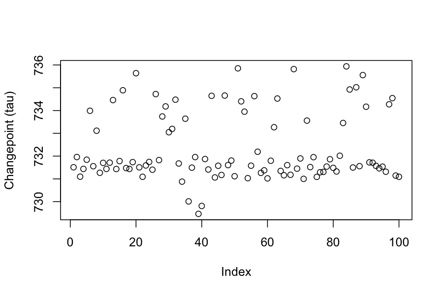
plot(extract(samples_changepoint)$tau, ylab = "Changepoint (tau)")

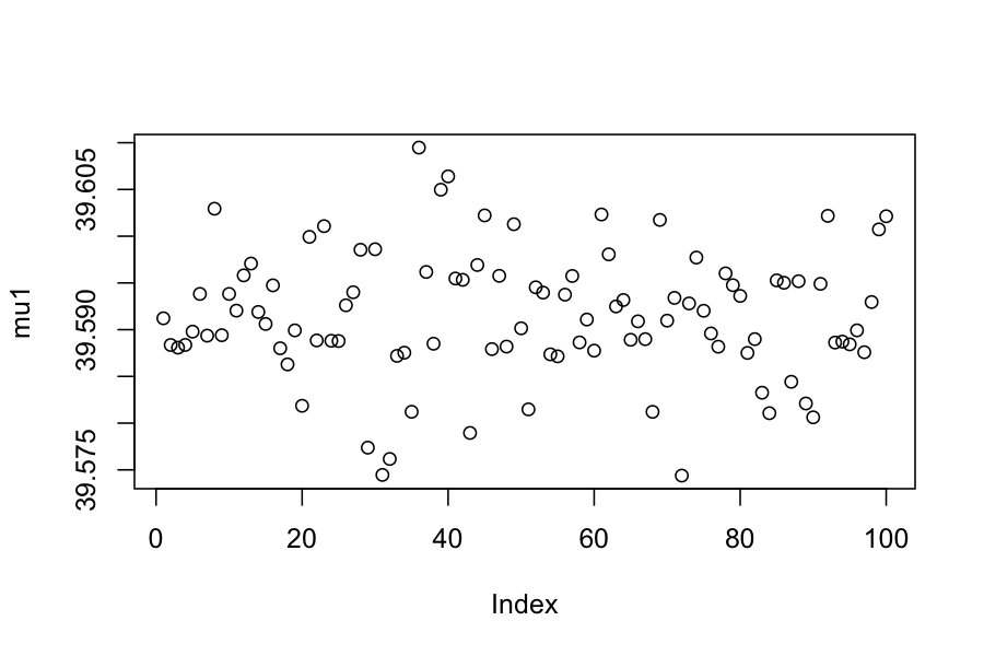
plot(extract(samples_changepoint)$mu[,1], ylab = "mu1")

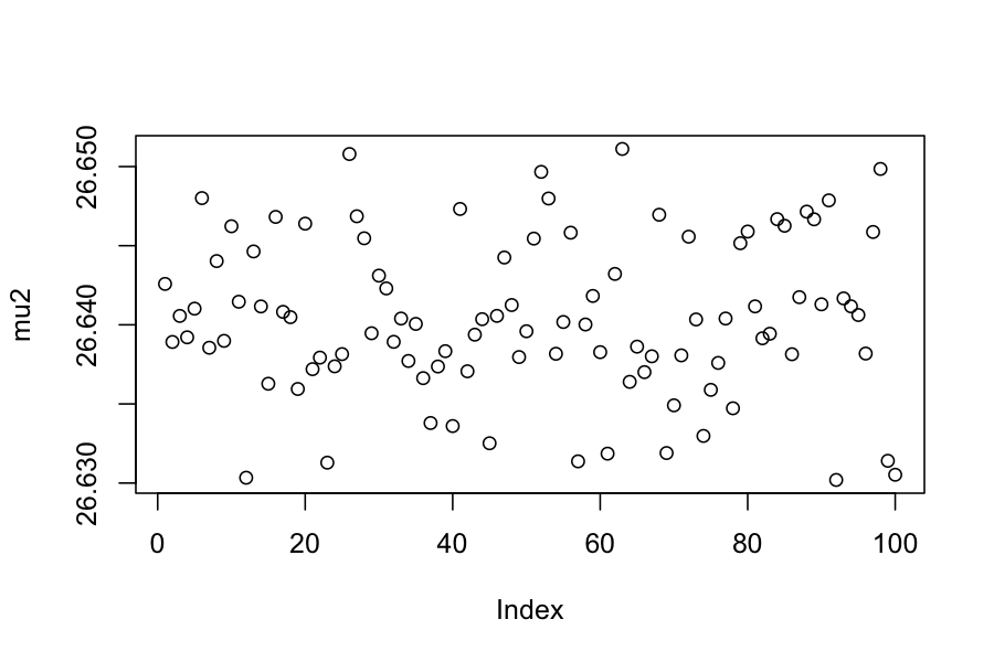
plot(extract(samples_changepoint)$mu[,2], ylab = "mu2")

(mean.tau <- mean(extract(samples_changepoint)$tau))

## [1] 732.3161

(mean.mu1 <- mean(extract(samples_changepoint)$mu[,1]))

## [1] 39.59149

(mean.mu2 <- mean(extract(samples_changepoint)$mu[,2]))

## [1] 26.6404

time_data <- data.frame(activity = c, time = 1:length(c))
time_data$activity_fitted <- ifelse(time_data$time <= mean.tau, mean.mu1, mean.mu2)
ggplot(time_data) + geom_point(aes(x = time, y = activity)) +
    geom_line(aes(x = time, y = activity_fitted), color = "red")

Lecture 26: MCMC Applications

The Bayesian Setup

The Bayesian Goal

Example 1: Estimating a correlation

Estimating a correlation with measurement error

Example 3: Seven scientists

Example 4: Changepoint detection

Summing up