Tidy data
We usually want our data in the folowing form:
Data don’t always come this way!
Even if the data do satisfy the “one row per observation” rule for
one analysis, they don’t necessarily do so for another, and we often
need to change the “shape” of the data.
Data semantics
Three concepts:
Values
Variables
Observations
Datasets contain values, each of which belongs to a
variable and an observation.
Datasets can encode these in a lot of different ways. The “tidy” way
is to have
Each variable a column
Each observation a row
Each cell a value
This is usually the way that other functions want the data to come
in.
For example:
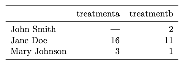
What is easy to do with data in this format?
What is hard to do with data in this format?
Same information:
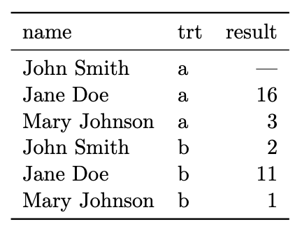
What is easy to do with data in this format?
What is hard?
Another example:
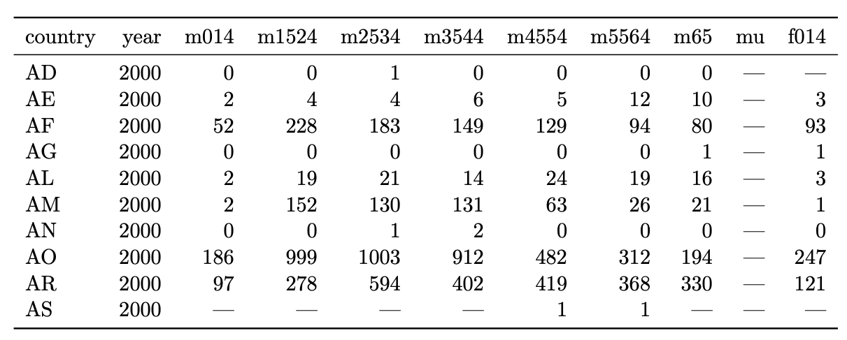
Easy:
Hard:
Plot cases as a function of sex, age, country, year.
Model cases as a function of sex, age, country, year.
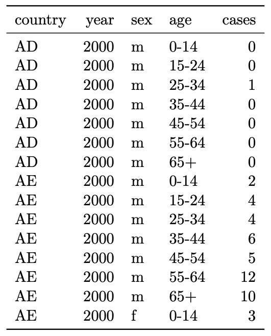
Easy:
Plot cases as a function of sex, age, country, year.
Model cases as a function of sex, age, country, year.
Hard:
Compute differences between number of cases in different
categories (e.g. differences in cases between males and females holding
all the other categories constant).
See overall number of cases (not as compact as the other
way).
General rules of thumb
Columns are all special (accessed by name) and rows are not
special (accessed programmatically).
Easy to define functional relationships between variables
(e.g. difference between two variables)/hard to define functional
relationships between rows.
Easy to subset rows/hard to subset columns.
Easy to aggregate over rows/hard to aggregate over
columns.
Reshaping
The term for transforming these datasets into each other is called
“reshaping”, and pretty much all reshaping can be done with a
combination of two operations: pivot_longer and
pivot_wider.
These two functions do essentially what their names imply:
You usually pivot_longer first to get the data into a
tidy, long form, and then pivot_wider if you need a
different layout for analysis or presentation.
Pivoting longer
The pivot_longer function takes data from wide form to
long form.
Syntax: pivot_longer(data, cols) or (usually)
data |> pivot_longer(cols)
data should be a data framecols the columns to pivot into longer form. The values
corresponding to these columns will all be put into one column in the
output dataset. Can be a character vector or something more complicated
that we will describe later.
What does the output look like?
- All the columns not listed in
cols remain as identifier
variables.
- One new column (called
name by default) stores the
former column names (the variable measured).
- Another new column (called
value by default) stores the
corresponding measurement values.
Pivoting longer examples
Let’s see an example. (Actually a very interesting study, can read here.)
##    time treatment subject rep potato buttery grassy rancid painty
## 61    1         1       3   1    2.9     0.0    0.0    0.0    5.5
## 25    1         1       3   2   14.0     0.0    0.0    1.1    0.0
## 62    1         1      10   1   11.0     6.4    0.0    0.0    0.0
## 26    1         1      10   2    9.9     5.9    2.9    2.2    0.0
## 63    1         1      15   1    1.2     0.1    0.0    1.1    5.1
## 27    1         1      15   2    8.8     3.0    3.6    1.5    2.3
We want to melt this data frame so that the “identification
variables” are time, treatment, subject, rep and the “measurement
variables” are the remainder: potato, buttery, grassy, rancid,
painty.
##
## Attaching package: 'tidyr'
## The following object is masked from 'package:reshape2':
##
##     smiths
french_fries_long <- french_fries |>
  pivot_longer(cols = c("potato", "buttery", "grassy", "rancid", "painty"))

head(french_fries_long)
## # A tibble: 6 × 6
##   time  treatment subject   rep name    value
##   <fct> <fct>     <fct>   <dbl> <chr>   <dbl>
## 1 1     1         3           1 potato    2.9
## 2 1     1         3           1 buttery   0
## 3 1     1         3           1 grassy    0
## 4 1     1         3           1 rancid    0
## 5 1     1         3           1 painty    5.5
## 6 1     1         3           2 potato   14
You can also specify columns using the column numbers (not
recommended) or same syntax that select
uses (much more useful). The following are all equivalent:
french_fries |>
    pivot_longer(cols = 5:9)
## # A tibble: 3,480 × 6
##    time  treatment subject   rep name    value
##    <fct> <fct>     <fct>   <dbl> <chr>   <dbl>
##  1 1     1         3           1 potato    2.9
##  2 1     1         3           1 buttery   0
##  3 1     1         3           1 grassy    0
##  4 1     1         3           1 rancid    0
##  5 1     1         3           1 painty    5.5
##  6 1     1         3           2 potato   14
##  7 1     1         3           2 buttery   0
##  8 1     1         3           2 grassy    0
##  9 1     1         3           2 rancid    1.1
## 10 1     1         3           2 painty    0
## # ℹ 3,470 more rows
french_fries |>
    pivot_longer(cols = c(potato, buttery, grassy, rancid, painty))
## # A tibble: 3,480 × 6
##    time  treatment subject   rep name    value
##    <fct> <fct>     <fct>   <dbl> <chr>   <dbl>
##  1 1     1         3           1 potato    2.9
##  2 1     1         3           1 buttery   0
##  3 1     1         3           1 grassy    0
##  4 1     1         3           1 rancid    0
##  5 1     1         3           1 painty    5.5
##  6 1     1         3           2 potato   14
##  7 1     1         3           2 buttery   0
##  8 1     1         3           2 grassy    0
##  9 1     1         3           2 rancid    1.1
## 10 1     1         3           2 painty    0
## # ℹ 3,470 more rows
french_fries |> pivot_longer(cols = potato:painty)
## # A tibble: 3,480 × 6
##    time  treatment subject   rep name    value
##    <fct> <fct>     <fct>   <dbl> <chr>   <dbl>
##  1 1     1         3           1 potato    2.9
##  2 1     1         3           1 buttery   0
##  3 1     1         3           1 grassy    0
##  4 1     1         3           1 rancid    0
##  5 1     1         3           1 painty    5.5
##  6 1     1         3           2 potato   14
##  7 1     1         3           2 buttery   0
##  8 1     1         3           2 grassy    0
##  9 1     1         3           2 rancid    1.1
## 10 1     1         3           2 painty    0
## # ℹ 3,470 more rows
french_fries |>
    pivot_longer(cols = -c(time, treatment, subject, rep))
## # A tibble: 3,480 × 6
##    time  treatment subject   rep name    value
##    <fct> <fct>     <fct>   <dbl> <chr>   <dbl>
##  1 1     1         3           1 potato    2.9
##  2 1     1         3           1 buttery   0
##  3 1     1         3           1 grassy    0
##  4 1     1         3           1 rancid    0
##  5 1     1         3           1 painty    5.5
##  6 1     1         3           2 potato   14
##  7 1     1         3           2 buttery   0
##  8 1     1         3           2 grassy    0
##  9 1     1         3           2 rancid    1.1
## 10 1     1         3           2 painty    0
## # ℹ 3,470 more rows
You can make the output slightly nicer by specifying variable names
and value names with names_to and
values_to:
french_fries |>
    pivot_longer(cols = potato:painty,
                 names_to = "flavor", values_to = "flavor_intensity")
## # A tibble: 3,480 × 6
##    time  treatment subject   rep flavor  flavor_intensity
##    <fct> <fct>     <fct>   <dbl> <chr>              <dbl>
##  1 1     1         3           1 potato               2.9
##  2 1     1         3           1 buttery              0
##  3 1     1         3           1 grassy               0
##  4 1     1         3           1 rancid               0
##  5 1     1         3           1 painty               5.5
##  6 1     1         3           2 potato              14
##  7 1     1         3           2 buttery              0
##  8 1     1         3           2 grassy               0
##  9 1     1         3           2 rancid               1.1
## 10 1     1         3           2 painty               0
## # ℹ 3,470 more rows
Pivoting wider
Syntax:
pivot_wider(data, id_cols, names_from, values_from, values_fn)
or, usually,
data |> pivot_wider(id_cols, names_from, values_from, values_fn)
data should be a data frame.id_cols specifies the variables you want to use to
define what the rows of the wide data frame should be.names_from specifies the variables you want to use to
define what the columns of the wide data frame sholud be.values_from specifies what the elements of the wide
data frame should be.values_fn: only used in some cases, discussed
later.
Example
french_fries_long = french_fries |>
    pivot_longer(cols = potato:painty,
                 names_to = "flavor", values_to = "flavor_intensity")
french_fries_long |>
    head()
## # A tibble: 6 × 6
##   time  treatment subject   rep flavor  flavor_intensity
##   <fct> <fct>     <fct>   <dbl> <chr>              <dbl>
## 1 1     1         3           1 potato               2.9
## 2 1     1         3           1 buttery              0
## 3 1     1         3           1 grassy               0
## 4 1     1         3           1 rancid               0
## 5 1     1         3           1 painty               5.5
## 6 1     1         3           2 potato              14
french_fries_long |>
    pivot_wider(id_cols = c(subject, rep, flavor),
                names_from = c(time, treatment),
                values_from = flavor_intensity) |>
    head()
## # A tibble: 6 × 33
##   subject   rep flavor  `1_1` `1_2` `1_3` `2_1` `2_2` `2_3` `3_1` `3_2` `3_3`
##   <fct>   <dbl> <chr>   <dbl> <dbl> <dbl> <dbl> <dbl> <dbl> <dbl> <dbl> <dbl>
## 1 3           1 potato    2.9  13.9  14.1   9    14.1   6.5  11.8   4     7.3
## 2 3           1 buttery   0     0     0     0.3   0.9   0.6   0.2   0.1   0.2
## 3 3           1 grassy    0     0     0     0.1   0.3   0.7   0     0     0
## 4 3           1 rancid    0     3.9   1.1   5.8   2.1   0.1   6     9.2   7.1
## 5 3           1 painty    5.5   0     0     0.3   0     1.4   0     0     0
## 6 3           2 potato   14    13.4   9.5   5.5   3.3  13.8   7.8   9.9   7.3
## # ℹ 21 more variables: `4_1` <dbl>, `4_2` <dbl>, `4_3` <dbl>, `5_1` <dbl>,
## #   `5_2` <dbl>, `5_3` <dbl>, `6_1` <dbl>, `6_2` <dbl>, `6_3` <dbl>,
## #   `7_1` <dbl>, `7_2` <dbl>, `7_3` <dbl>, `8_1` <dbl>, `8_2` <dbl>,
## #   `8_3` <dbl>, `9_1` <dbl>, `9_2` <dbl>, `9_3` <dbl>, `10_1` <dbl>,
## #   `10_2` <dbl>, `10_3` <dbl>
french_fries_long |> subset(time == 1 & subject == "3" & rep == 1 & flavor == "potato")
## # A tibble: 3 × 6
##   time  treatment subject   rep flavor flavor_intensity
##   <fct> <fct>     <fct>   <dbl> <chr>             <dbl>
## 1 1     1         3           1 potato              2.9
## 2 1     2         3           1 potato             13.9
## 3 1     3         3           1 potato             14.1
If you don’t specify id_cols, pivot_wider
assumes that everything that is not specified in names_from
and values_from should be used as id_cols.
french_fries_long |>
    pivot_wider(id_cols = c(subject, rep, flavor),
                names_from = c(time, treatment),
                values_from = flavor_intensity) |>
    head()
## # A tibble: 6 × 33
##   subject   rep flavor  `1_1` `1_2` `1_3` `2_1` `2_2` `2_3` `3_1` `3_2` `3_3`
##   <fct>   <dbl> <chr>   <dbl> <dbl> <dbl> <dbl> <dbl> <dbl> <dbl> <dbl> <dbl>
## 1 3           1 potato    2.9  13.9  14.1   9    14.1   6.5  11.8   4     7.3
## 2 3           1 buttery   0     0     0     0.3   0.9   0.6   0.2   0.1   0.2
## 3 3           1 grassy    0     0     0     0.1   0.3   0.7   0     0     0
## 4 3           1 rancid    0     3.9   1.1   5.8   2.1   0.1   6     9.2   7.1
## 5 3           1 painty    5.5   0     0     0.3   0     1.4   0     0     0
## 6 3           2 potato   14    13.4   9.5   5.5   3.3  13.8   7.8   9.9   7.3
## # ℹ 21 more variables: `4_1` <dbl>, `4_2` <dbl>, `4_3` <dbl>, `5_1` <dbl>,
## #   `5_2` <dbl>, `5_3` <dbl>, `6_1` <dbl>, `6_2` <dbl>, `6_3` <dbl>,
## #   `7_1` <dbl>, `7_2` <dbl>, `7_3` <dbl>, `8_1` <dbl>, `8_2` <dbl>,
## #   `8_3` <dbl>, `9_1` <dbl>, `9_2` <dbl>, `9_3` <dbl>, `10_1` <dbl>,
## #   `10_2` <dbl>, `10_3` <dbl>
french_fries_long |>
    pivot_wider(names_from = c(time, treatment),
                values_from = flavor_intensity) |>
    head()
## # A tibble: 6 × 33
##   subject   rep flavor  `1_1` `1_2` `1_3` `2_1` `2_2` `2_3` `3_1` `3_2` `3_3`
##   <fct>   <dbl> <chr>   <dbl> <dbl> <dbl> <dbl> <dbl> <dbl> <dbl> <dbl> <dbl>
## 1 3           1 potato    2.9  13.9  14.1   9    14.1   6.5  11.8   4     7.3
## 2 3           1 buttery   0     0     0     0.3   0.9   0.6   0.2   0.1   0.2
## 3 3           1 grassy    0     0     0     0.1   0.3   0.7   0     0     0
## 4 3           1 rancid    0     3.9   1.1   5.8   2.1   0.1   6     9.2   7.1
## 5 3           1 painty    5.5   0     0     0.3   0     1.4   0     0     0
## 6 3           2 potato   14    13.4   9.5   5.5   3.3  13.8   7.8   9.9   7.3
## # ℹ 21 more variables: `4_1` <dbl>, `4_2` <dbl>, `4_3` <dbl>, `5_1` <dbl>,
## #   `5_2` <dbl>, `5_3` <dbl>, `6_1` <dbl>, `6_2` <dbl>, `6_3` <dbl>,
## #   `7_1` <dbl>, `7_2` <dbl>, `7_3` <dbl>, `8_1` <dbl>, `8_2` <dbl>,
## #   `8_3` <dbl>, `9_1` <dbl>, `9_2` <dbl>, `9_3` <dbl>, `10_1` <dbl>,
## #   `10_2` <dbl>, `10_3` <dbl>
Aggregation
When you pivot wider, you don’t necessarily use all of the
variables.
This means that each element of the cast table will correspond to
more than one measurement, and so they need to be aggregated in some
way.
## # A tibble: 6 × 6
##   time  treatment subject   rep flavor  flavor_intensity
##   <fct> <fct>     <fct>   <dbl> <chr>              <dbl>
## 1 1     1         3           1 potato               2.9
## 2 1     1         3           1 buttery              0
## 3 1     1         3           1 grassy               0
## 4 1     1         3           1 rancid               0
## 5 1     1         3           1 painty               5.5
## 6 1     1         3           2 potato              14
french_fries_long |>
    pivot_wider(id_cols = time,
                names_from = flavor,
                values_from = flavor_intensity)
## Warning: Values from `flavor_intensity` are not uniquely identified; output will contain list-cols.
## • Use `values_fn = list` to suppress this warning.
## • Use `values_fn = {summary_fun}` to summarise duplicates.
## • Use the following dplyr code to identify duplicates.
##   {data} |>
##   dplyr::summarise(n = dplyr::n(), .by = c(time, flavor)) |>
##   dplyr::filter(n > 1L)
## # A tibble: 10 × 6
##    time  potato     buttery    grassy     rancid     painty
##    <fct> <list>     <list>     <list>     <list>     <list>
##  1 1     <dbl [72]> <dbl [72]> <dbl [72]> <dbl [72]> <dbl [72]>
##  2 2     <dbl [72]> <dbl [72]> <dbl [72]> <dbl [72]> <dbl [72]>
##  3 3     <dbl [72]> <dbl [72]> <dbl [72]> <dbl [72]> <dbl [72]>
##  4 4     <dbl [72]> <dbl [72]> <dbl [72]> <dbl [72]> <dbl [72]>
##  5 5     <dbl [72]> <dbl [72]> <dbl [72]> <dbl [72]> <dbl [72]>
##  6 6     <dbl [72]> <dbl [72]> <dbl [72]> <dbl [72]> <dbl [72]>
##  7 7     <dbl [72]> <dbl [72]> <dbl [72]> <dbl [72]> <dbl [72]>
##  8 8     <dbl [72]> <dbl [72]> <dbl [72]> <dbl [72]> <dbl [72]>
##  9 9     <dbl [60]> <dbl [60]> <dbl [60]> <dbl [60]> <dbl [60]>
## 10 10    <dbl [60]> <dbl [60]> <dbl [60]> <dbl [60]> <dbl [60]>
You can use the values_fn argument to
pivot_wider to define how to aggregate values.
french_fries_long |>
    pivot_wider(id_cols = time,
                names_from = flavor,
                values_from = flavor_intensity,
                values_fn = mean)
## # A tibble: 10 × 6
##    time  potato buttery grassy rancid painty
##    <fct>  <dbl>   <dbl>  <dbl>  <dbl>  <dbl>
##  1 1       8.56    2.24  0.942   2.36   1.65
##  2 2       8.06    2.72  1.18    2.85   1.44
##  3 3       7.80    2.10  0.75    3.72   1.31
##  4 4       7.71    1.80  0.742   3.60   1.37
##  5 5      NA      NA    NA      NA     NA
##  6 6       6.67    1.75  0.674   4.08   2.34
##  7 7       6.17   NA     0.421   3.89   2.68
##  8 8       5.43   NA     0.381   4.27  NA
##  9 9       5.67    1.59  0.277   4.67   3.87
## 10 10      5.70    1.76  0.557   6.07   5.29
french_fries_long |>
    pivot_wider(names_from = flavor,
                id_cols = time,
                values_from = flavor_intensity,
                values_fn = function(x) mean(x))
## # A tibble: 10 × 6
##    time  potato buttery grassy rancid painty
##    <fct>  <dbl>   <dbl>  <dbl>  <dbl>  <dbl>
##  1 1       8.56    2.24  0.942   2.36   1.65
##  2 2       8.06    2.72  1.18    2.85   1.44
##  3 3       7.80    2.10  0.75    3.72   1.31
##  4 4       7.71    1.80  0.742   3.60   1.37
##  5 5      NA      NA    NA      NA     NA
##  6 6       6.67    1.75  0.674   4.08   2.34
##  7 7       6.17   NA     0.421   3.89   2.68
##  8 8       5.43   NA     0.381   4.27  NA
##  9 9       5.67    1.59  0.277   4.67   3.87
## 10 10      5.70    1.76  0.557   6.07   5.29
french_fries_long |>
    pivot_wider(names_from = flavor,
                id_cols = time,
                values_from = flavor_intensity,
                values_fn = function(x) mean(x, na.rm = TRUE))
## # A tibble: 10 × 6
##    time  potato buttery grassy rancid painty
##    <fct>  <dbl>   <dbl>  <dbl>  <dbl>  <dbl>
##  1 1       8.56    2.24  0.942   2.36   1.65
##  2 2       8.06    2.72  1.18    2.85   1.44
##  3 3       7.80    2.10  0.75    3.72   1.31
##  4 4       7.71    1.80  0.742   3.60   1.37
##  5 5       7.33    1.64  0.635   3.53   2.02
##  6 6       6.67    1.75  0.674   4.08   2.34
##  7 7       6.17    1.37  0.421   3.89   2.68
##  8 8       5.43    1.18  0.381   4.27   3.94
##  9 9       5.67    1.59  0.277   4.67   3.87
## 10 10      5.70    1.76  0.557   6.07   5.29
The tidyverse functions also have shortcut notation for
defining anonymous functions. See here
for details. It works best for functions that have one or two arguments,
which are referred to as .x (first/only argument) and
.y (second argument in a two-argument function).
## "shortcut" version
french_fries_long |>
    pivot_wider(names_from = flavor,
                id_cols = time,
                values_from = flavor_intensity,
                values_fn = ~mean(.x, na.rm = TRUE))
## # A tibble: 10 × 6
##    time  potato buttery grassy rancid painty
##    <fct>  <dbl>   <dbl>  <dbl>  <dbl>  <dbl>
##  1 1       8.56    2.24  0.942   2.36   1.65
##  2 2       8.06    2.72  1.18    2.85   1.44
##  3 3       7.80    2.10  0.75    3.72   1.31
##  4 4       7.71    1.80  0.742   3.60   1.37
##  5 5       7.33    1.64  0.635   3.53   2.02
##  6 6       6.67    1.75  0.674   4.08   2.34
##  7 7       6.17    1.37  0.421   3.89   2.68
##  8 8       5.43    1.18  0.381   4.27   3.94
##  9 9       5.67    1.59  0.277   4.67   3.87
## 10 10      5.70    1.76  0.557   6.07   5.29
Merging
Final topic: What if you have data from two different places and you
need to put them together?
Base R syntax: merge(x, y, by.x, by.y)
x and y are the two datasets you want
to merge.
by.x is the column of x to merge
on.
by.y is the column of y to merge
on.
dpylr syntax:
*_join(x, y, by = c("x_col" = "y_col"))
*_join can be any of left_join,
right_join, inner_join, full_join
for different types of merges.
by argument is a character vector specifying the
columns to join on.
Defaults to matching all columns with the same name.
Example:
cities <- data.frame(
    city=c('New York','Boston','Juneau',
           'Anchorage','San Diego',
           'Philadelphia','Los Angeles',
           'Fairbanks','Ann Arbor','Seattle'),
    state.abb=c('NY','MA','AK','AK','CA',
                'PA','CA','AK','MI','WA'))

states <- data.frame(state.name, state.abb)
cities
##            city state.abb
## 1      New York        NY
## 2        Boston        MA
## 3        Juneau        AK
## 4     Anchorage        AK
## 5     San Diego        CA
## 6  Philadelphia        PA
## 7   Los Angeles        CA
## 8     Fairbanks        AK
## 9     Ann Arbor        MI
## 10      Seattle        WA
##   state.name state.abb
## 1    Alabama        AL
## 2     Alaska        AK
## 3    Arizona        AZ
## 4   Arkansas        AR
## 5 California        CA
## 6   Colorado        CO
We want to add the state name to the cities data frame, and we can
use merge.
##
## Attaching package: 'dplyr'
## The following objects are masked from 'package:stats':
##
##     filter, lag
## The following objects are masked from 'package:base':
##
##     intersect, setdiff, setequal, union
## base R
merge(states, cities, by.x = "state.abb", by.y = "state.abb")
##    state.abb    state.name         city
## 1         AK        Alaska       Juneau
## 2         AK        Alaska    Anchorage
## 3         AK        Alaska    Fairbanks
## 4         CA    California    San Diego
## 5         CA    California  Los Angeles
## 6         MA Massachusetts       Boston
## 7         MI      Michigan    Ann Arbor
## 8         NY      New York     New York
## 9         PA  Pennsylvania Philadelphia
## 10        WA    Washington      Seattle
## dplyr
inner_join(states, cities, by = "state.abb")
##       state.name state.abb         city
## 1         Alaska        AK       Juneau
## 2         Alaska        AK    Anchorage
## 3         Alaska        AK    Fairbanks
## 4     California        CA    San Diego
## 5     California        CA  Los Angeles
## 6  Massachusetts        MA       Boston
## 7       Michigan        MI    Ann Arbor
## 8       New York        NY     New York
## 9   Pennsylvania        PA Philadelphia
## 10    Washington        WA      Seattle
Notice in the last example that there was some ambiguity in how the
merge took place because the two datasets have different sets of values
for state.abb.
In base R, the default is an inner join (you get one row for each
value of the merging variable that was seen in both x and
y)
Modify with all, all.x,
all.y:
all = TRUE is a full outer join (you get one row for
values of the merging variable that were seen in either x
or y)
all.x = TRUE is a left join (you get one row for
each value of the merging variable that was seen in
x)
all.y = TRUE is a right join (you get one row for
each value of the merging variable that was seen in
y)
In dplyr, you use inner_join,
outer_join, left_join,
right_join
merge(states, cities, all.x = TRUE)
##    state.abb     state.name         city
## 1         AK         Alaska       Juneau
## 2         AK         Alaska    Anchorage
## 3         AK         Alaska    Fairbanks
## 4         AL        Alabama         <NA>
## 5         AR       Arkansas         <NA>
## 6         AZ        Arizona         <NA>
## 7         CA     California    San Diego
## 8         CA     California  Los Angeles
## 9         CO       Colorado         <NA>
## 10        CT    Connecticut         <NA>
## 11        DE       Delaware         <NA>
## 12        FL        Florida         <NA>
## 13        GA        Georgia         <NA>
## 14        HI         Hawaii         <NA>
## 15        IA           Iowa         <NA>
## 16        ID          Idaho         <NA>
## 17        IL       Illinois         <NA>
## 18        IN        Indiana         <NA>
## 19        KS         Kansas         <NA>
## 20        KY       Kentucky         <NA>
## 21        LA      Louisiana         <NA>
## 22        MA  Massachusetts       Boston
## 23        MD       Maryland         <NA>
## 24        ME          Maine         <NA>
## 25        MI       Michigan    Ann Arbor
## 26        MN      Minnesota         <NA>
## 27        MO       Missouri         <NA>
## 28        MS    Mississippi         <NA>
## 29        MT        Montana         <NA>
## 30        NC North Carolina         <NA>
## 31        ND   North Dakota         <NA>
## 32        NE       Nebraska         <NA>
## 33        NH  New Hampshire         <NA>
## 34        NJ     New Jersey         <NA>
## 35        NM     New Mexico         <NA>
## 36        NV         Nevada         <NA>
## 37        NY       New York     New York
## 38        OH           Ohio         <NA>
## 39        OK       Oklahoma         <NA>
## 40        OR         Oregon         <NA>
## 41        PA   Pennsylvania Philadelphia
## 42        RI   Rhode Island         <NA>
## 43        SC South Carolina         <NA>
## 44        SD   South Dakota         <NA>
## 45        TN      Tennessee         <NA>
## 46        TX          Texas         <NA>
## 47        UT           Utah         <NA>
## 48        VA       Virginia         <NA>
## 49        VT        Vermont         <NA>
## 50        WA     Washington      Seattle
## 51        WI      Wisconsin         <NA>
## 52        WV  West Virginia         <NA>
## 53        WY        Wyoming         <NA>
left_join(states, cities, by = "state.abb")
##        state.name state.abb         city
## 1         Alabama        AL         <NA>
## 2          Alaska        AK       Juneau
## 3          Alaska        AK    Anchorage
## 4          Alaska        AK    Fairbanks
## 5         Arizona        AZ         <NA>
## 6        Arkansas        AR         <NA>
## 7      California        CA    San Diego
## 8      California        CA  Los Angeles
## 9        Colorado        CO         <NA>
## 10    Connecticut        CT         <NA>
## 11       Delaware        DE         <NA>
## 12        Florida        FL         <NA>
## 13        Georgia        GA         <NA>
## 14         Hawaii        HI         <NA>
## 15          Idaho        ID         <NA>
## 16       Illinois        IL         <NA>
## 17        Indiana        IN         <NA>
## 18           Iowa        IA         <NA>
## 19         Kansas        KS         <NA>
## 20       Kentucky        KY         <NA>
## 21      Louisiana        LA         <NA>
## 22          Maine        ME         <NA>
## 23       Maryland        MD         <NA>
## 24  Massachusetts        MA       Boston
## 25       Michigan        MI    Ann Arbor
## 26      Minnesota        MN         <NA>
## 27    Mississippi        MS         <NA>
## 28       Missouri        MO         <NA>
## 29        Montana        MT         <NA>
## 30       Nebraska        NE         <NA>
## 31         Nevada        NV         <NA>
## 32  New Hampshire        NH         <NA>
## 33     New Jersey        NJ         <NA>
## 34     New Mexico        NM         <NA>
## 35       New York        NY     New York
## 36 North Carolina        NC         <NA>
## 37   North Dakota        ND         <NA>
## 38           Ohio        OH         <NA>
## 39       Oklahoma        OK         <NA>
## 40         Oregon        OR         <NA>
## 41   Pennsylvania        PA Philadelphia
## 42   Rhode Island        RI         <NA>
## 43 South Carolina        SC         <NA>
## 44   South Dakota        SD         <NA>
## 45      Tennessee        TN         <NA>
## 46          Texas        TX         <NA>
## 47           Utah        UT         <NA>
## 48        Vermont        VT         <NA>
## 49       Virginia        VA         <NA>
## 50     Washington        WA      Seattle
## 51  West Virginia        WV         <NA>
## 52      Wisconsin        WI         <NA>
## 53        Wyoming        WY         <NA>
merge(states, cities, all.y = TRUE)
##    state.abb    state.name         city
## 1         AK        Alaska       Juneau
## 2         AK        Alaska    Anchorage
## 3         AK        Alaska    Fairbanks
## 4         CA    California    San Diego
## 5         CA    California  Los Angeles
## 6         MA Massachusetts       Boston
## 7         MI      Michigan    Ann Arbor
## 8         NY      New York     New York
## 9         PA  Pennsylvania Philadelphia
## 10        WA    Washington      Seattle
right_join(states, cities, by = "state.abb")
##       state.name state.abb         city
## 1         Alaska        AK       Juneau
## 2         Alaska        AK    Anchorage
## 3         Alaska        AK    Fairbanks
## 4     California        CA    San Diego
## 5     California        CA  Los Angeles
## 6  Massachusetts        MA       Boston
## 7       Michigan        MI    Ann Arbor
## 8       New York        NY     New York
## 9   Pennsylvania        PA Philadelphia
## 10    Washington        WA      Seattle
merge(states, cities, all = TRUE)
##    state.abb     state.name         city
## 1         AK         Alaska       Juneau
## 2         AK         Alaska    Anchorage
## 3         AK         Alaska    Fairbanks
## 4         AL        Alabama         <NA>
## 5         AR       Arkansas         <NA>
## 6         AZ        Arizona         <NA>
## 7         CA     California    San Diego
## 8         CA     California  Los Angeles
## 9         CO       Colorado         <NA>
## 10        CT    Connecticut         <NA>
## 11        DE       Delaware         <NA>
## 12        FL        Florida         <NA>
## 13        GA        Georgia         <NA>
## 14        HI         Hawaii         <NA>
## 15        IA           Iowa         <NA>
## 16        ID          Idaho         <NA>
## 17        IL       Illinois         <NA>
## 18        IN        Indiana         <NA>
## 19        KS         Kansas         <NA>
## 20        KY       Kentucky         <NA>
## 21        LA      Louisiana         <NA>
## 22        MA  Massachusetts       Boston
## 23        MD       Maryland         <NA>
## 24        ME          Maine         <NA>
## 25        MI       Michigan    Ann Arbor
## 26        MN      Minnesota         <NA>
## 27        MO       Missouri         <NA>
## 28        MS    Mississippi         <NA>
## 29        MT        Montana         <NA>
## 30        NC North Carolina         <NA>
## 31        ND   North Dakota         <NA>
## 32        NE       Nebraska         <NA>
## 33        NH  New Hampshire         <NA>
## 34        NJ     New Jersey         <NA>
## 35        NM     New Mexico         <NA>
## 36        NV         Nevada         <NA>
## 37        NY       New York     New York
## 38        OH           Ohio         <NA>
## 39        OK       Oklahoma         <NA>
## 40        OR         Oregon         <NA>
## 41        PA   Pennsylvania Philadelphia
## 42        RI   Rhode Island         <NA>
## 43        SC South Carolina         <NA>
## 44        SD   South Dakota         <NA>
## 45        TN      Tennessee         <NA>
## 46        TX          Texas         <NA>
## 47        UT           Utah         <NA>
## 48        VA       Virginia         <NA>
## 49        VT        Vermont         <NA>
## 50        WA     Washington      Seattle
## 51        WI      Wisconsin         <NA>
## 52        WV  West Virginia         <NA>
## 53        WY        Wyoming         <NA>
full_join(states, cities, by = "state.abb")
##        state.name state.abb         city
## 1         Alabama        AL         <NA>
## 2          Alaska        AK       Juneau
## 3          Alaska        AK    Anchorage
## 4          Alaska        AK    Fairbanks
## 5         Arizona        AZ         <NA>
## 6        Arkansas        AR         <NA>
## 7      California        CA    San Diego
## 8      California        CA  Los Angeles
## 9        Colorado        CO         <NA>
## 10    Connecticut        CT         <NA>
## 11       Delaware        DE         <NA>
## 12        Florida        FL         <NA>
## 13        Georgia        GA         <NA>
## 14         Hawaii        HI         <NA>
## 15          Idaho        ID         <NA>
## 16       Illinois        IL         <NA>
## 17        Indiana        IN         <NA>
## 18           Iowa        IA         <NA>
## 19         Kansas        KS         <NA>
## 20       Kentucky        KY         <NA>
## 21      Louisiana        LA         <NA>
## 22          Maine        ME         <NA>
## 23       Maryland        MD         <NA>
## 24  Massachusetts        MA       Boston
## 25       Michigan        MI    Ann Arbor
## 26      Minnesota        MN         <NA>
## 27    Mississippi        MS         <NA>
## 28       Missouri        MO         <NA>
## 29        Montana        MT         <NA>
## 30       Nebraska        NE         <NA>
## 31         Nevada        NV         <NA>
## 32  New Hampshire        NH         <NA>
## 33     New Jersey        NJ         <NA>
## 34     New Mexico        NM         <NA>
## 35       New York        NY     New York
## 36 North Carolina        NC         <NA>
## 37   North Dakota        ND         <NA>
## 38           Ohio        OH         <NA>
## 39       Oklahoma        OK         <NA>
## 40         Oregon        OR         <NA>
## 41   Pennsylvania        PA Philadelphia
## 42   Rhode Island        RI         <NA>
## 43 South Carolina        SC         <NA>
## 44   South Dakota        SD         <NA>
## 45      Tennessee        TN         <NA>
## 46          Texas        TX         <NA>
## 47           Utah        UT         <NA>
## 48        Vermont        VT         <NA>
## 49       Virginia        VA         <NA>
## 50     Washington        WA      Seattle
## 51  West Virginia        WV         <NA>
## 52      Wisconsin        WI         <NA>
## 53        Wyoming        WY         <NA>
Some additional notes:
Default if you don’t specify by.x and
by.y is to use the columns that are common to the
two.
by.x/by.y can have length more than 1,
in which case we match on the entire set of specified
variables.
Can use by instead of by.x and
by.y, in which case the name of the column to merge on has
to be the same in both x and y.
cities <- data.frame(
  city = c("New York", "Boston", "Juneau", "Anchorage", "San Diego"),
  state.abb = c("NY", "MA", "AK", "AK", "CA"),
  year = c(2020, 2020, 2021, 2021, 2020)
)


population <- data.frame(
  abb = c("NY", "MA", "AK", "AK", "CA"),
  year = c(2020, 2020, 2021, 2020, 2020),
  pop_million = c(19.3, 6.9, 0.7, 0.73, 39.5)
)

cities
##        city state.abb year
## 1  New York        NY 2020
## 2    Boston        MA 2020
## 3    Juneau        AK 2021
## 4 Anchorage        AK 2021
## 5 San Diego        CA 2020
##   abb year pop_million
## 1  NY 2020       19.30
## 2  MA 2020        6.90
## 3  AK 2021        0.70
## 4  AK 2020        0.73
## 5  CA 2020       39.50
Notice that cities and population have
different names for the column giving the state abbreviation.
Below we see an example of merging on two columns in base R and in
dplyr when the column names are not the same in the two datasets.
merge(cities, population, by.x = c("state.abb", "year"), by.y = c("abb", "year"))
##   state.abb year      city pop_million
## 1        AK 2021    Juneau         0.7
## 2        AK 2021 Anchorage         0.7
## 3        CA 2020 San Diego        39.5
## 4        MA 2020    Boston         6.9
## 5        NY 2020  New York        19.3
inner_join(cities, population, by = c("state.abb" = "abb", "year" = "year"))
##        city state.abb year pop_million
## 1  New York        NY 2020        19.3
## 2    Boston        MA 2020         6.9
## 3    Juneau        AK 2021         0.7
## 4 Anchorage        AK 2021         0.7
## 5 San Diego        CA 2020        39.5