Monte Carlo methods: integration and cross validation

Agenda today: Simulation-based methods of computing expectations

Monte Carlo integration
Cross validation

Reading: Lange 21.1, 21.2, 21.6

Monte Carlo Integration

We have:

A function $f$
A distribution $\mu$

We would like to approximate \[ E[f(X)] = \int f(x) \, d\mu(x) \]

Why not numerical integration?

Works well for low-dimensional problems.
Fails in high dimensions, the “curse of dimensionality”

Monte Carlo Integration

To estimate/approximate \[ E[f(X)] = \int f(x) \, d\mu(x) \]

Draw $X_1, \ldots, X_n$ iid from $\mu$
Use $\frac{1}{n} \sum_{i=1}^n f(X_i)$ as the estimator

Why is this reasonable?

By the law of large numbers, the estimates converge to $E[f(X)]$ as $n \to \infty$

Monte Carlo Integration: Accuracy

If $f$ is square integrable, we can apply the central limit theorem, which tells us that the estimator is approximately distributed \[ \mathcal N \left( E[f(X)], \sqrt{\frac{\text{Var}[f(X)]}{n}} \right) \]

Good thing: accuracy doesn’t depend on the dimensionality of the problem
Bad thing: Error declines at the $n^{-1/2}$ rate vs. $n^{-k}$, $k \ge 2$ for the numerical integration methods.
What to do? Try to decrease $\text{Var}[f(X)]$.

Importance Sampling

Importance sampling is based on the following equality: \[ \int f(x) g(x)\, d \nu (x) = \int \frac{f(x) g(x)}{h(x)} h(x) \,d \nu(x) \] where

$f$ is the function for which we would like to compute the expectation
$\nu$ is some base measure (Lebesgue or counting)
$g$ is the density of our target probability distribution relative to $\nu$ (so the measure $\mu$ from before is $g d \nu$).
$h$ is the density of some other probability distribution relative to $\nu$

Importance sampling: Procedure

Draw $Y_1, \ldots, Y_n$ iid from a distribution $h$. Then \[ \frac{1}{n}\sum_{i=1}^n \frac{f(Y_i) g(Y_i)}{h(Y_i)} \] is an estimate of $\int f(x) g(x) \, d \nu(x)$.

When is this useful?

The importance sampling estimator has a smaller variance than the naive estimator iff: \[ \int \left[ \frac{f(x) g(x)}{h(x)} \right]^2 h(x) d\nu(x) \le \int f(x)^2 g(x) d\nu(x) \]

If we choose $h(x) = |f(x)| g(x) / \int |f(z)| g(z) d\nu(z)$, then an application of Cauchy Schwarz tells us that the condition above is satisfied and the importance sampling estimator will have smaller variance.

If $f$ is nonnegative and $h$ is chosen as above, the variance of the importance sampling estimator is 0.

We aren’t able to choose $h$ according to the recipe above, but it implies that the variance will be reduced if $h(x)$ looks like $|f(x)| g(x)$.

A contrived example

We are playing a terrible game:

I draw from a uniform distribution on $[0,1]$.
If the draw comes up less than $.01$, you have to pay me $100.
Otherwise nothing happens.

What is your expected return to playing this game?

Naive Monte Carlo estimate:

set.seed(1)
f = function(x) {
    if(x < .01)
        return(-100)
    return(0)
}
mc_samples = runif(1000)
mean(sapply(mc_samples, f))

## [1] -0.7

Not very good!
Problem is that we don’t have very many samples where $x < .01$
Try importance sampling from a distribution that is more likely to give $x < .01$

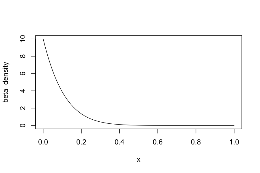
Recall Beta distributions: Supported on the interval $[0,1]$, can tune so that they put more weight in the middle or at the edges.

Beta(1,10) has density:

x = seq(0, 1, length.out = 200)
beta_density = dbeta(x, shape1 = 1, shape2 = 10)
plot(beta_density ~ x, type = 'l')

Importance sampling from Beta(1,10):

mc_importance_samples = rbeta(1000, shape1 = 1, shape2 = 10)
importance_function = function(x) {
    return(f(x) / dbeta(x, shape1 = 1, shape2 = 10))
}
mean(sapply(mc_importance_samples, importance_function))

## [1] -1.044691

More realistic examples

Intuition from the game holds: if you have extreme returns from rare events, importance sampling by sampling more from regions with extreme returns helps
Insurance
Quantitative finance

Rao-Blackwellization

Let $\tau(U, X)$ be an estimator of some function

Then \[ \text{var}(\tau(U, X)) = \text{var}[E[\tau(U, X) | X]] + E[\text{var}(\tau(U, X) | X)] \] which means that $\tau' = E[\tau(U, X) \mid X]$ has a smaller variance than $\tau$

“Rao-Blackwellization” for Monte Carlo Integration using the Accept/Reject algorithm

Setup:

We want to estimate $E[f(X)] = \int f(x) g(x) \, dx$
We have some $h$, $c$ such that $g(x) \le ch(x)$
We generate $N$ points $X_1,\ldots, X_N$ from $h(x)$
We generate $N$ points $U_1,\ldots, U_N$ from a standard uniform.
We accept $X_i$ if $U_i \le W_i = g(X_i) / [ch(X_i)]$.
$N$ is a random number so that we have $m$ acceptances.

The Monte Carlo estimator of $E[f(X)]$ is \[ \frac{1}{m} \sum_{i=1}^N \mathbf 1_{\{U_i \le W_i\}} f(X_i) \]

Can we condition?

\[ \begin{align*} \frac{1}{m} E&\left[ \sum_{i=1}^N \mathbf 1_{\{U_i \le W_i\}} f(X_i) | N, X_1,\ldots, X_N \right] \\ &= \frac{1}{m}\sum_{i=1}^N E\left[ \mathbf 1_{\{U_i \le W_i\}} | N, W_1,\ldots, W_N\right] f(X_i) \end{align*} \]

$E \left[ \mathbf 1_{\{U_i \le W_i\}} | N, W_1,\ldots, W_N \right]$ is the probability that we accept $X_i$ given that we sample $N$ deviates and accept $m$ of them

If $m$, $N$ are large, we will have

\[ E \left[ \mathbf 1_{\{U_i \le W_i\}} | N, W_1,\ldots, W_N \right] \approx W_i m / N \approx W_i / c \]

Example:

$h$ the standard uniform distribution, $c = 10$

one_rb_sample = function() {
    c = 10
    X = runif(1)
    U = runif(1)
    W = dbeta(X, shape1 = 1, shape2 = 10) / (c * dunif(X))
    return(c(accepted = (U <= W), fX = f(X), weight = W / c))
}
samples = replicate(n = 10000, one_rb_sample())
m = sum(samples["accepted",])
fX = samples["fX",]
weights = samples["weight",]
sum(fX * weights) / m

## [1] -0.9477492

Part 2: Cross validation

We have:

Data $X_1, \ldots, X_n$.
A tuning parameter $\theta$. Each value of $\theta$ corresponds to a different set of models.
A function $L$ that takes a fitted model and a data point and returns a measure of model quality.

We would like to choose one model from the set of candidate models indexed by $\theta$.

Example: Regression

Data: Pairs of predictors and response variables, $(y_i, X_i)$, $i = 1,\ldots, n$, $y_i \in \mathbb R$, $X_i \in \mathbb R^p$
Models: $y_i = X \beta + \epsilon$, $\beta_j = 0, j \in S_\theta$, where $S_\theta \subseteq \{1,\ldots, p\}$.
Model quality: Squared-error loss. If $\hat \beta_\theta$ are our estimates of the regression coefficients in model $\theta$, model quality is measured by \[ L(\hat \beta_\theta, (y_i, X_i)) = (y_i - X_i^T \hat \beta_\theta)^2 \]

We want to choose a subset of the predictors that do the best job of explaining the response.

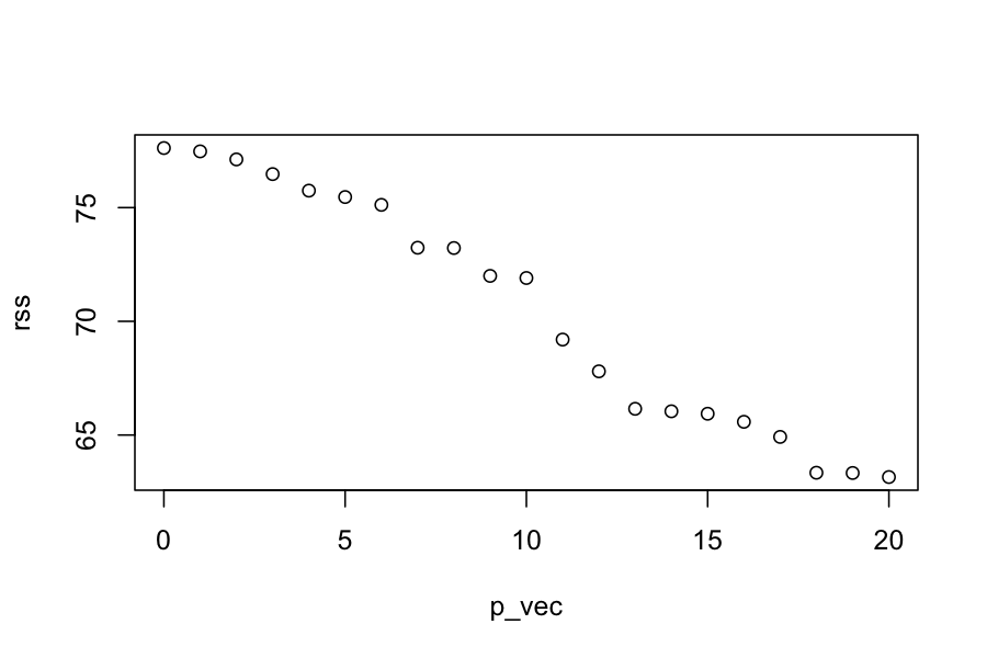
Naive solution: Find the model that has the lowest value for the squared-error loss.

Why doesn’t this work?

Example: Mixture models

Data: $x_1,\ldots, x_n$, $x_i \in \mathbb R$
Models: Gaussian mixture models with $\theta$ mixture components.
Model quality: Negative log likelihood of the data. If $\hat p_\theta$ is the density of the fitted model with $\theta$ components, model quality is measured by $L(\hat p_\theta, x_i) = -\log \hat p_\theta(x_i)$.

We want to choose the number of mixture components that best explains the data.

Naive solution: Choose the number of mixture components that minimizes the negative log likelihood of the data.

Better Solution: Cross validation

Idea: Instead of measuring model quality on the same data we used to fit the model, we estimate model quality on new data.

If we knew the true distribution of the data, we could simulate new data and use a Monte Carlo estimate based on the simulations.

We can’t actually get new data, and so we hold some back when we fit the model and then pretend that the held back data is new data.

Procedure:

Divide the data into $K$ folds
Let $X^{(k)}$ denote the data in fold $k$, and let $X^{(-k)}$ denote the data in all the folds except for $k$.
For each fold and each value of the tuning parameter $\theta$, fit the model on $X^{(-k)}$ to get $\hat f_\theta^{(k)}$
Compute \[ \text{CV}(\theta) = \frac{1}{n} \sum_{k=1}^K \sum_{x \in X^{(k)}} L(\hat f_\theta^{(k)}, x) \]
Choose $\hat \theta = \text{argmin}_{\theta} \text{CV}(\theta)$

Example

n = 100
p = 20
X = matrix(rnorm(n * p), nrow = n)
y = rnorm(n)
get_rss_submodels = function(n_predictors, y, X) {
    if(n_predictors == 0) {
        lm_submodel = lm(y ~ 0)
    } else {
        lm_submodel = lm(y ~ 0 + X[,1:n_predictors, drop = FALSE])
    }
    return(sum(residuals(lm_submodel)^2))
}
p_vec = 0:p
rss = sapply(p_vec, get_rss_submodels, y, X)
plot(rss ~ p_vec)

get_cv_error = function(n_predictors, y, X, folds) {
    cv_vec = numeric(length(unique(folds)))
    for(f in unique(folds)) {
        cv_vec[f] = rss_on_held_out(
                  n_predictors,
                  y_train = y[folds != f],
                  X_train = X[folds != f,],
                  y_test = y[folds == f],
                  X_test = X[folds == f,])
    }
    return(mean(cv_vec))
}

rss_on_held_out = function(n_predictors, y_train, X_train, y_test, X_test) {
    if(n_predictors == 0) {
        lm_submodel = lm(y_train ~ 0)
        preds_on_test = rep(0, length(y_test))
    } else {
        lm_submodel = lm(y_train ~ 0 + X_train[,1:n_predictors, drop = FALSE])
        preds_on_test = X_test[,1:n_predictors, drop= FALSE] %*% coef(lm_submodel)
    }

    return(sum((y_test - preds_on_test)^2))
}
K = 5
## normally you would do this at random
folds = rep(1:K, each = n / K)
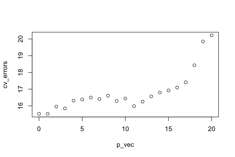
p_vec = 0:p
cv_errors = sapply(p_vec, get_cv_error, y, X, folds)
plot(cv_errors ~ p_vec)

Choice of $K$

Considerations:

Larger $K$ means more computation (although sometimes there is a shortcut for leave-one-out cross validation)
Larger $K$ means less bias in the estimate of model accuracy
Larger $K$ also means more variance in the estimate, so we don’t necessarily want $K = n$
Usually choose $K = 5$ or $K = 10$
If your problem is structured (e.g. time series, spatial), you should choose the folds to respect the structure.

Summing up

We can use simulations to estimate arbitrary functions of our random variables.
If we know the underlying distribution, we can simply simulate from it (Monte Carlo integration).
If we don’t know the underlying distribution, we can “simulate” from the data by resampling from the data (cross validation). Resampling methods will do well to the extent that the observed data reflect the true data-generating distribution.

Monte Carlo methods: integration and cross validation

Monte Carlo Integration

Monte Carlo Integration

Monte Carlo Integration: Accuracy

Importance Sampling

Importance sampling: Procedure

When is this useful?

A contrived example

More realistic examples

Rao-Blackwellization

“Rao-Blackwellization” for Monte Carlo Integration using the Accept/Reject algorithm

Part 2: Cross validation

Example: Regression

Example: Mixture models

Better Solution: Cross validation

Example

Choice of \(K\)

Summing up