Generating random deviates
Logistics
Makeup office hours tomorrow 10am-12pm
I’ll set up a discussion board on canvas where you can ask questions of me, John, and your classmates
Agenda for today
Reading:
Random numbers vs pseudo-random numbers
True randomness: From nature
On computers: Everything deterministic, so we only have pseudo-random number generators
Functions that produce a sequence of numbers that have some of the same properties of a sequence of independent uniform random variables
They cannot have all of the properties of a sequence of independent uniform random variables
Issue tends to be independence rather than uniformity
e.g. the linear congruential generator
Linear congruential generator
A generator, so it makes a sequence of numbers.
Start off with \(X_0\).
Define \(X_{n+1} = (aX_n + c) \text{ mod } m\)
- \(m\), \(0<m\) is the “modulus”
- \(a\), \(0 < a < m\) — the “multiplier”
- \(c\), \(0 \le c < m\) — the “increment”
- \(X_0\), \(0 \le X_0 < m\) — the “seed” or “start value”
lcg_sequence = function(a=5, c=12, m=16, seed = 10, n_deviates = 20) {
    sequence = numeric(n_deviates)
    sequence[1] = seed
    for(i in 2:n_deviates) {
        sequence[i] = (a * sequence[i-1] + c) %% m
    }
  return(sequence)
}
lcg_sequence()
## [1] 10 14 2 6 10 14 2 6 10 14 2 6 10 14 2 6 10 14 2 6
## [1] 4 0 12 8 4 0 12 8 4 0 12 8 4 0 12 8 4 0 12 8
Small values of \(m\), \(a\), \(c\) give sequences with relatively small period (time before the sequence repeats).
One recommendation:
random_unifs = (lcg_sequence(a = 25214903917, c = 11, m = 2^48, seed = 2^47 - 17, n_deviates = 1000)) /
    2^48
head(round(random_unifs, digits = 3))
## [1] 0.500 0.498 0.715 0.444 0.353 0.458
## [1] 0.507
## [1] 0.804
## [1] 0.179
Problem setup
We have
A (pseudo) random number generator that provides us with independent, uniformly distributed random numbers
A probability distribution with CDF \(F\)
We want
- A sequence of independent \(F\)-distributed random numbers
Inverse method
Let
\[
F^{[-1]}(y) = \text{inf}\{x : F(x) \ge y\}, \quad y \in [0,1]
\]
If \(F\) is strictly increasing, we have \(F^{[-1]} = F^{-1}\).
Intuition:
Suppose \(F\) strictly increasing, \(F^{-1}\) exists, \(U \sim \text{Unif}(0,1)\).
Then \(F^{-1}(U) \sim F\).
Why?
\[
\begin{align*}
P(F^{-1}(U) \le x) &= P(F(F^{-1}(U)) \le F(x)) \\
&= P(U \le F(x)) \\
&= F(x)
\end{align*}
\]
And so the CDF of \(F^{-1}(U)\) is \(F(x)\)
Inverse method: Procedure
Let \(F\) be the CDF of the target distribution, and let \[
F^{[-1]}(y) = \text{inf}\{x : F(x) \ge y\}, \quad y \in [0,1]
\]
Inverse method: Exponential distribution
CDF for a random variable distributed exponential with rate 1:
\[
F(x) = 1 - e^{-x}
\]
\[
F^{[-1]}(u) = -\log(1 - u)
\]
\(F\) is strictly increasing and continuous, so just check that \(F(F^{-1}(u)) = u\).
Algorithm:
Note: We can also take \(X = -\log(U)\). Why?
Let’s check:
generate_exponential = function() {
    U = runif(1)
    X = -log(1 - U)
    return(X)
}
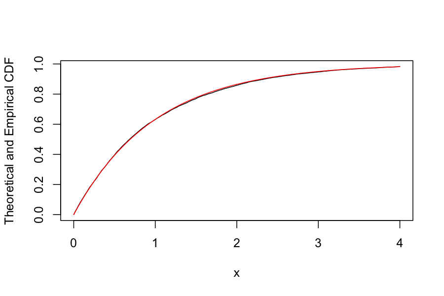
random_exponentials = replicate(n = 10000, generate_exponential())
grid = seq(0,4, length.out = 200)
plot(sapply(grid, function(g) mean(random_exponentials <= g)) ~ grid, type = 'l',
     ylab = "Theoretical and Empirical CDF", xlab = "x")
points(pexp(grid) ~ grid, type = 'l', col = "red")

Let’s check:
generate_discrete_uniform = function(n) {
    U = runif(1)
    return(floor(n * U) + 1)
}
discrete_uniforms = replicate(n = 10000, generate_discrete_uniform(3))
head(discrete_uniforms)
## [1] 1 3 3 1 1 1
table(discrete_uniforms) / length(discrete_uniforms)
## discrete_uniforms
##      1      2      3
## 0.3330 0.3332 0.3338
Acceptance-Rejection Method
Problem setup:
Acceptance-Rejection Procedure
Sample \(U \sim \text{Uniform}[0,1]\) and \(Z \sim g\)
If \(U \le \frac{f(Z)}{ c g(Z)}\), return \(Z\)
Otherwise, return to 1
Acceptance-Rejection Method: Why does it work?
Probability of generating an accepted value in \((x, x + dx)\) is proportional to \[
g(x) dx \frac{f(x)}{h(x)} = \frac{1}{c} f(x) dx
\]
\(g(x)\) gives the probability of proposing something in \((x, x + dx)\)
\(f(x) / h(x)\) is the probability of accepting the proposal
Overall idea: Think of \(g\) as approximating \(f\), and \(f(x) / h(x)\) as describing how well \(h\) approximates \(f\) at \(x\). We accept more of the time when \(f(x) / h(x)\) is large.
Notes
The expected number of iterations required to accept a draw is \(1/c\)
Therefore, should make \(c\) as small as possible
\(f\) doesn’t have to be a normalized density
Acceptance-Rejection Method: Example
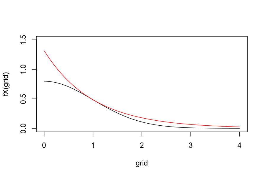
We want \(X\) with density \[
f_X(x) = \frac{2}{\sqrt{2\pi}} e^{-x^2 / 2}, \quad x \ge 0
\]
Let \(g(x) = e^{-x}\), \(x \ge 0\) (exponential with rate 1)
Let \(c = \sqrt {2e / \pi} \approx 1.32\) (obtained by finding the maximum of \(f_X(x) / g(x)\))
Check: \(f_X(x) \le cg(x)\) for all \(x \ge 0\)
fX = function(x) 2 / sqrt(2 * pi) * exp(-x^2 / 2)
g = function(x) exp(-x)
c = sqrt(2 * exp(1) / pi)
grid = seq(0, 4, length.out = 200)
plot(fX(grid) ~ grid, type = 'l', ylim = c(0, 1.5))
points(c * g(grid) ~ grid, type = 'l', col = 'red')

Overall algorithm:
Generate \(Z \sim \text{Exp}(1)\)
Generate \(U \sim \text{Unif}(0,1)\)
If \(U \le \frac{f_X(Z)}{ c g(Z)} = \frac{2}{\sqrt{e}}\exp(-Z^2 / 2 + Z)\), return \(Z\)
Let’s check:
gen_half_normal = function() {
    while(TRUE) {
        U = runif(1)
        Z = rexp(1, rate = 1)
        if(U <= fX(Z) / (c * g(Z))) {
            return(Z)
        }
    }
}
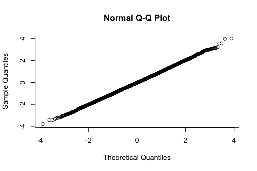
half_normals = replicate(n = 10000, gen_half_normal())
signs = ifelse(runif(10000) >= .5, -1, 1)
normals = half_normals * signs
qqnorm(normals)

Why might we want to do this?
Maybe we actually want half normals.
Can use half normals to make standard normals, standard normals to make arbitrary normals.
Summing up
For simulation, we tend to use pseudo-random number generators
Pseudo-random number generators target a uniform distribution
Many methods for generating random numbers from other distributions
Inverse method for when you have the CDF and it is easy to invert
Accept/Reject for more complicated distributions, and for which you don’t know or want to compute the normalizing constant.
