Applications and cvx
Agenda today
Convex optimization problem
In a convex optimization problem, we minimize a convex function over a convex set.
Standard form for an optimization problem is:
\[
\begin{align*}
\text{minimize} \quad &f_0(x) \\
\text{subject to}\quad &f_i(x) \le 0, \quad i = 1,\ldots, m\\
&a_j^T x = b_j, \quad j = 1,\ldots, n
\end{align*}
\]
\(x \in \mathbb R^n\) is the optimization variable
\(f_0: \mathbb R^n \to \mathbb R\) is the objective function
\(f_i : \mathbb R^n \to \mathbb R\) are the inequality constraint functions
\(a_j^T x = b_j\) are the equality constraints
Regression
Standard least squares problem is convex: \[
\text{minimize} \|y - X \beta\|_2^2
\]
Regularized regression
Any “regularization” with a convex function \(P\) will still be convex:
\[
\text{minimize} \|y - X \beta\|_2^2 + P(\beta)
\]
Covariance estimation
Let \(S\) denote the sample covariance and \(\Theta\) be the inverse covariance matrix.
Up to constant factors, the log-likelihood of the data given a Gaussian distribution is
\[
\log \det \Theta - \text{tr}(S \Theta)
\]
Covariance estimation would be by maximizing the log likelihood or minimizing the negative log likelihood.
\(\log \det\) is concave, \(\text{tr}(S \Theta)\) is linear
Restriction of \(\Theta\) to be positive definite is a restriction to a convex set
Convex problem; remains convex if we add convex penalties to \(\Theta\)
Summing up
If you can show an optimization problem is convex, you’re very likely able to solve it efficiently
Many statistical estimation problems are naturally convex
You have a couple of options for checking convexity:
Check the definition
Check first-order conditions (not usually as useful)
Check second-order conditions (good option if the function is differentiable)
Check restriction to a line
Check whether the function can be re-expressed as a combination of convex functions and convexity-preserving operations
Defining an optimization problem in cvx
Remember how we defined a convex optimization problem:
\[
\begin{align*}
\text{minimize} \quad &f_0(x) \\
\text{subject to}\quad &f_i(x) \le 0, \quad i = 1,\ldots, m\\
&a_j^T x = b_j, \quad j = 1,\ldots, n
\end{align*}
\]
Components:
Variables to minimize over (\(x\) in the formulation above, can be multi-dimensional)
Objective function (\(f_0\) above, what we want to minimize)
Constraints on the variables
In the cvx package, we define these three components, create a problem out of them, and the solver will do the rest.
Example
For example, suppose our problem is: \[
\begin{align*}
\text{minimize}_{x, y} \quad &x^2 + y^2 \\
\text{subject to} \quad &x \ge 0\\
& 2x + y = 1
\end{align*}
\]
How do we set this up in cvx/R?
Define the variables to be minimized over:
##
## Attaching package: 'CVXR'
## The following object is masked from 'package:stats':
##
##     power
# Variables minimized over
x = Variable(1)
y = Variable(1)
x
## Variable(1, 1)
## [1] "Variable"
## attr(,"package")
## [1] "CVXR"
Define the objective function:
# The function we want to minimize
objective = Minimize(x^2 + y^2)
objective
## An object of class "Minimize"
## Slot "expr":
## AddExpression(c("Expression(CONVEX, POSITIVE, 1)", "Expression(CONVEX, POSITIVE, 1)"), c("Expression(CONVEX, POSITIVE, 1)", "Expression(CONVEX, POSITIVE, 1)"))
## [1] "Minimize"
## attr(,"package")
## [1] "CVXR"
Define the constraints:
## The constraints
constraints = list(x >= 0, 2*x + y == 1)
constraints
## [[1]]
## LeqConstraint(Constant(CONSTANT, ZERO, (1,1)), Variable(1, 1))
## [[2]]
## EqConstraint(Expression(AFFINE, UNKNOWN, 1), Expression(AFFINE, UNKNOWN, 1), Constant(CONSTANT, POSITIVE, (1,1)))
The optimization problem is then composed of the objective and the constraints:
## Problem definition
prob <- Problem(objective, constraints)
To perform the optimization we use solve(problem)
# Problem solution
solution = solve(prob)
solution$status
## [1] "optimal"
## [1] 0.3999978
## [1] 0.2000044
## check that the solution satisfies the constraints
solution$getValue(x) >= 0
## [1] TRUE
2 * solution$getValue(x) + solution$getValue(y)
## [1] 1
Least squares
We’ll start off with the least squares problem and work up to more elaborate problems.
We are doing regression, so we have a response variable \(y \in \mathbb R^n\) and predictor variables stored as the rows of a matrix \(X \in \mathbb R^{n \times p}\).
The least squares problem is \[
\text{minimize}_{\beta} \|y - X \beta\|_2^2
\] or, written without matrix notation: \[
\text{minimize}_{\beta} \sum_{i=1}^n (y_i - \sum_{j=1}^pX_{ij} \beta_j)^2
\]
This is a very simple convex optimization problem, just an objective function to be minimized, no constraints on the parameters.
Example dataset
The data set dating (in lattice.RData) contains paired observations giving the estimated ages of 19 coral samples in thousands of years using both carbon dating (the traditional method) and thorium dating (a modern and purportedly more accurate method.)
We want to know about the difference between these two methods.
We can set this up as a linear model:
load("lattice.RData")
dating_lm = lm(thorium - carbon ~ carbon, data = dating)
round(coef(dating_lm), digits = 2)
## (Intercept)      carbon
##        0.14        0.16
Let’s try to solve the same problem with cvx.
First set up the data:
y = dating$thorium - dating$carbon
X = cbind(1, dating$carbon)
Define the optimization variables:
Define the objective function:
objective = Minimize(sum((y - X %*% betahat)^2))
Solve the problem and get the fitted values:
problem = Problem(objective)
result = solve(problem)
round(result$getValue(betahat), digits = 2)
##      [,1]
## [1,] 0.14
## [2,] 0.16
round(coef(dating_lm), digits = 2)
## (Intercept)      carbon
##        0.14        0.16
Robust Regression
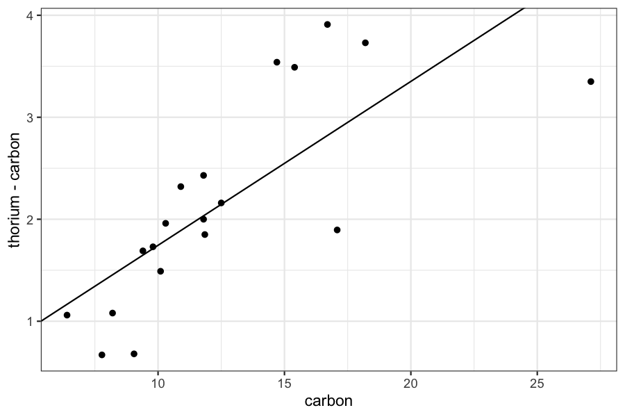
If we look more carefully at our data, we see that there appear to be some outliers: most of the points follow one trend line, and the other two are far off.
This means that the least squares line doesn’t do a good job of capturing either the bulk of the data or the outliers.
To deal with this situation, we sometimes use robust regression.
ggplot(dating) + geom_point(aes(x = carbon, y = thorium - carbon)) +
    geom_abline(aes(intercept = result$getValue(betahat)[1], slope = result$getValue(betahat)[2]))

Robust regression is a modification of least squares that is meant to deal with outliers.
The coefficients in the Huber version of robust regression are the solutions to the problem \[
\text{minimize}_\beta \quad \sum_{i=1}^n H(y_i - \sum_{j=1}^p X_{ij} \beta_j, M)
\] where \(H\) is the Huber loss function: \[
H(z, M) = \begin{cases}
z^2 & z\le M \\
2M|z| - M^2 & z > M
\end{cases}
\]
Let’s set up the problem in cvx.
Define the variables to optimize over:
Define the objective function
objective = Minimize(sum(huber(y - X %*% betahat, M = .46)))
Solve the problem and get the fitted values for the regression coefficients:
problem = Problem(objective)
result = solve(problem)
result$getValue(betahat)
##            [,1]
## [1,] -0.4452392
## [2,]  0.2162504
fitted_betahat = result$getValue(betahat)
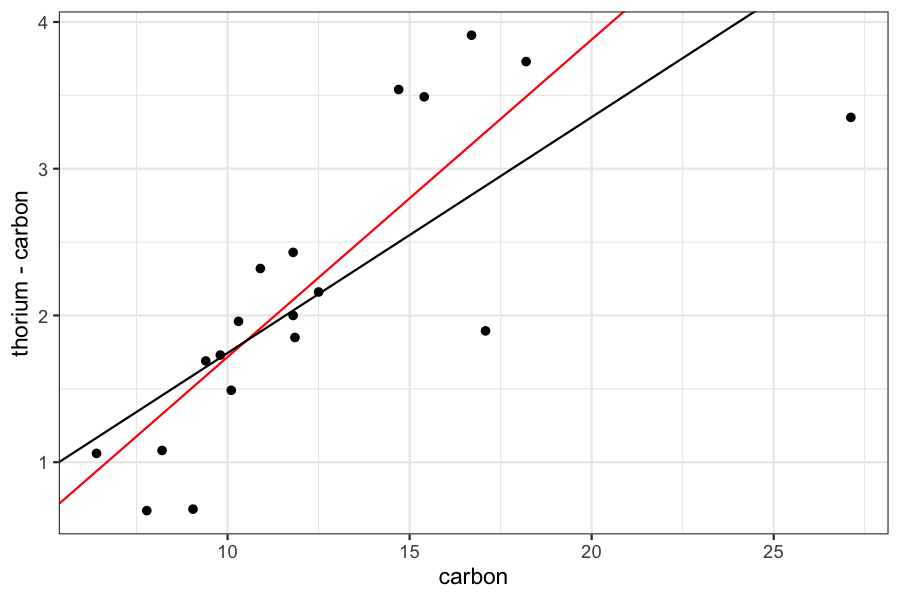
Compare the regression line from robust regression to the standard regression line:
ggplot(dating) + geom_point(aes(x = carbon, y = thorium - carbon)) +
    geom_abline(aes(slope = fitted_betahat[2], intercept = fitted_betahat[1]), color = 'red') +
    geom_abline(aes(slope = coef(dating_lm)[2], intercept = coef(dating_lm)[1]))

Variable selection
A popular way of doing variable selection in high-dimensional regression problems is with the lasso.
The Lasso is a simple modification of the least squares problem: \[
\text{minimize}_{\beta} \sum_{i=1}^n (y_i - \sum_{j=1}^p X_{ij} \beta_j)^2 + \lambda\sum_{j=1}^p |\beta_j|
\]
The resulting coefficient vector tends to be “sparse”, with many of the coefficients being estimated as exactly 0.
This is helpful when you want a model for your response that only incorporates a subset of the predictors.
Diabetes example
Ten baseline variables: age, sex, bmi, average blood pressure, plus six blood serum measurements.
Want to use this to predict “a quantitative measure of disease progression” in 442 patients.
We don’t necessarily think that all of the measured variables are important, and we want to get a model that uses only a subset of the variables but still gives us good predictive accuracy.
This is exactly what the lasso is for!
First set up the data:
## Loaded lars 1.2
data(diabetes)
head(diabetes$x)
## [1]  0.038075906 -0.001882017  0.085298906 -0.089062939  0.005383060
## [6] -0.092695478
## re-doing this because diabetes has a funny class
X = matrix(diabetes$x, nrow = nrow(diabetes$x), ncol = ncol(diabetes$x))
## changing X so each column has mean 0 and standard deviation 1
X = scale(X)
Y = diabetes$y
n = nrow(X)
p = ncol(X)
Let’s set up the problem in cvx. Define the variables:
Define the objective function:
lambda = 1
objective = Minimize(sum(n^(-1) * (Y - X %*% beta_lasso)^2) + lambda * sum(abs(beta_lasso)))
Define the problem and solve:
problem = Problem(objective)
result = solve(problem)
round(result$getValue(beta_lasso), digits = 2)
##         [,1]
##  [1,]  -0.03
##  [2,] -10.35
##  [3,]  25.01
##  [4,]  14.70
##  [5,]  -7.89
##  [6,]   0.00
##  [7,]  -8.38
##  [8,]   3.45
##  [9,]  24.98
## [10,]   2.95
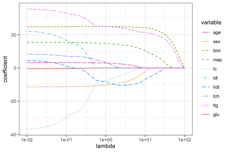
Let’s look at what happens to the coefficients with different values of \(\lambda\):
lambda_search = 10^(seq(-2, 2, length.out = 40))
get_beta_hat_lasso = function(lambda) {
    objective = Minimize(sum(n^(-1) * (Y - X %*% beta_lasso)^2) + lambda * sum(abs(beta_lasso)))
    problem = Problem(objective)
    result = solve(problem)
    result$getValue(beta_lasso)
}
beta_hats = plyr::aaply(lambda_search, 1, get_beta_hat_lasso)
colnames(beta_hats) = colnames(diabetes$x)
beta_hats = cbind(lambda = lambda_search, beta_hats)
round(beta_hats, digits = 2)
##    lambda   age    sex   bmi   map     tc   ldl    hdl  tch   ltg  glu
## 1    0.01 -0.47 -11.41 24.76 15.44 -36.95 22.11   4.44 8.29 35.50 3.22
## 2    0.01 -0.47 -11.41 24.76 15.44 -36.81 22.00   4.36 8.26 35.45 3.22
## 3    0.02 -0.46 -11.40 24.76 15.43 -36.47 21.74   4.21 8.21 35.33 3.22
## 4    0.02 -0.46 -11.40 24.76 15.43 -36.15 21.50   4.06 8.15 35.21 3.22
## 5    0.03 -0.45 -11.40 24.77 15.42 -35.69 21.14   3.84 8.07 35.04 3.22
## 6    0.03 -0.44 -11.39 24.77 15.41 -35.22 20.78   3.61 7.98 34.88 3.22
## 7    0.04 -0.44 -11.38 24.77 15.40 -34.50 20.23   3.26 7.85 34.62 3.22
## 8    0.05 -0.43 -11.37 24.78 15.39 -33.63 19.56   2.85 7.70 34.31 3.21
## 9    0.07 -0.41 -11.36 24.78 15.38 -32.53 18.71   2.32 7.51 33.91 3.21
## 10   0.08 -0.39 -11.34 24.79 15.36 -31.14 17.64   1.66 7.27 33.41 3.21
## 11   0.11 -0.37 -11.32 24.81 15.33 -29.48 16.35   0.88 6.99 32.81 3.21
## 12   0.13 -0.34 -11.29 24.82 15.31 -27.74 14.98   0.11 6.75 32.17 3.20
## 13   0.17 -0.32 -11.24 24.84 15.29 -27.06 14.35  -0.03 6.84 31.89 3.19
## 14   0.22 -0.28 -11.16 24.89 15.25 -25.81 13.22  -0.31 6.96 31.37 3.16
## 15   0.27 -0.24 -11.09 24.92 15.20 -22.92 10.90  -1.52 6.64 30.30 3.15
## 16   0.35 -0.17 -11.00 24.97 15.13 -19.02  7.77  -3.15 6.20 28.85 3.12
## 17   0.44 -0.09 -10.89 25.03 15.05 -14.05  3.80  -5.25 5.62 27.01 3.10
## 18   0.55 -0.03 -10.75 25.08 14.96  -9.22  0.02  -7.33 4.96 25.24 3.07
## 19   0.70 -0.03 -10.61 25.06 14.87  -8.75  0.00  -7.70 4.43 25.15 3.02
## 20   0.89  0.00 -10.42 25.03 14.75  -8.16  0.00  -8.16 3.75 25.04 2.96
## 21   1.13  0.00 -10.19 24.99 14.61  -7.43  0.00  -8.72 2.90 24.91 2.88
## 22   1.43  0.00  -9.90 24.94 14.44  -6.51  0.00  -9.44 1.85 24.74 2.78
## 23   1.80  0.00  -9.55 24.89 14.21  -5.43  0.00 -10.23 0.65 24.54 2.67
## 24   2.29  0.00  -9.09 24.83 13.97  -4.55  0.00 -10.56 0.01 24.26 2.45
## 25   2.89  0.00  -8.56 24.76 13.69  -3.91  0.00 -10.39 0.00 23.87 2.20
## 26   3.67  0.00  -7.91 24.68 13.34  -3.11 -0.02 -10.20 0.00 23.36 1.92
## 27   4.64  0.00  -7.02 24.58 12.90  -2.05  0.00  -9.88 0.00 22.76 1.43
## 28   5.88  0.00  -5.93 24.45 12.33  -0.74  0.00  -9.53 0.00 21.98 0.89
## 29   7.44  0.00  -4.52 24.36 11.60   0.00  0.00  -8.76 0.00 21.49 0.36
## 30   9.43  0.00  -2.70 24.27 10.63   0.00  0.00  -7.44 0.00 21.32 0.03
## 31  11.94  0.00  -0.54 24.08  9.37   0.00  0.00  -5.82 0.00 20.98 0.00
## 32  15.12  0.00   0.00 23.55  8.29   0.00  0.00  -4.61 0.00 20.45 0.00
## 33  19.14  0.00   0.00 22.77  7.08   0.00  0.00  -3.39 0.00 19.74 0.00
## 34  24.24  0.00   0.00 21.77  5.57   0.00  0.00  -1.88 0.00 18.83 0.00
## 35  30.70  0.00   0.00 20.49  3.61   0.00  0.00  -0.07 0.00 17.64 0.00
## 36  38.88  0.00   0.00 18.32  1.27   0.00  0.00   0.00 0.00 15.47 0.00
## 37  49.24  0.00   0.00 15.08  0.00   0.00  0.00   0.00 0.00 12.22 0.00
## 38  62.36  0.00   0.00 10.54  0.00   0.00  0.00   0.00 0.00  7.68 0.00
## 39  78.97  0.00   0.00  4.76  0.00   0.00  0.00   0.00 0.00  1.95 0.00
## 40 100.00  0.00   0.00  0.00  0.00   0.00  0.00   0.00 0.00  0.00 0.00
Plot of the coefficients for different values of \(\lambda\):
beta_melted = reshape2::melt(data.frame(beta_hats), id.vars = "lambda", value.name = "coefficient")
ggplot(beta_melted) +
    geom_line(aes(x = lambda, y = coefficient, color = variable, lty = variable)) +
    scale_x_log10()

Both together now!
What if we want to do both robust regression (we’re worried about outliers or corrupted data) and variable selection?
We can use the Huber loss on the residuals and the lasso penalty on the coefficients: \[
\text{minimize}_{\beta} \sum_{i=1}^n H(y_i - \sum_{j=1}^pX_{ij}\beta_j, M)+ \lambda \sum_{j=1}^p |\beta_j|
\]
I don’t know if there’s an actual implementation of this in an R package, but it’s easy to do with cvx.
Define the variable to be optimized over:
Define the objective:
lambda = 10^(-4)
objective = Minimize(sum(huber(Y - X %*% betahat)) + lambda * sum(abs(betahat)))
Define the problem and solve it:
problem = Problem(objective)
result = solve(problem)
round(result$getValue(betahat), digits = 2)
##       [,1]
##  [1,] 0.00
##  [2,] 0.00
##  [3,] 0.71
##  [4,] 0.00
##  [5,] 0.00
##  [6,] 0.00
##  [7,] 0.00
##  [8,] 0.00
##  [9,] 1.31
## [10,] 0.00
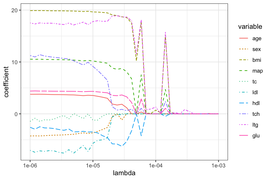
Searching over a grid of \(\lambda\):
lambda_search = 10^(seq(-6, -3, length.out = 40))
get_beta_hat_lasso = function(lambda) {
    objective = Minimize(sum(huber(Y - X %*% beta_lasso)) + lambda * sum(abs(beta_lasso)))
    problem = Problem(objective)
    result = solve(problem)
    result$getValue(beta_lasso)
}
beta_hats = plyr::aaply(lambda_search, 1, get_beta_hat_lasso)
colnames(beta_hats) = colnames(diabetes$x)
beta_hats = cbind(lambda = lambda_search, beta_hats)
round(beta_hats, digits = 2)
##    lambda  age   sex   bmi   map    tc   ldl   hdl   tch   ltg  glu
## 1       0 3.78 -4.26 19.91 10.54 -1.45 -7.03 -2.60 11.24 17.53 4.39
## 2       0 3.78 -4.25 19.92 10.51 -0.86 -7.41 -2.96 10.97 17.34 4.42
## 3       0 3.79 -4.26 19.91 10.54 -1.46 -7.14 -2.49 11.41 17.53 4.39
## 4       0 3.76 -4.21 19.91 10.48 -1.15 -7.24 -2.71 11.15 17.45 4.39
## 5       0 3.73 -4.15 19.87 10.48 -1.18 -7.08 -2.74 11.01 17.49 4.37
## 6       0 3.71 -4.11 19.87 10.46 -0.99 -7.16 -2.84 10.90 17.44 4.36
## 7       0 3.71 -4.10 19.87 10.45 -0.60 -7.43 -3.03 10.80 17.31 4.36
## 8       0 3.69 -4.05 19.86 10.43 -0.32 -7.57 -3.17 10.67 17.22 4.35
## 9       0 3.66 -4.00 19.83 10.41 -0.99 -6.91 -2.93 10.59 17.50 4.34
## 10      0 3.65 -3.94 19.82 10.37  0.07 -7.59 -3.49 10.23 17.14 4.34
## 11      0 3.58 -3.80 19.77 10.30 -0.42 -6.85 -3.44  9.82 17.41 4.31
## 12      0 3.51 -3.66 19.73 10.23 -0.92 -6.12 -3.37  9.43 17.68 4.27
## 13      0 3.58 -3.79 19.77 10.31  0.01 -7.28 -3.50  9.95 17.20 4.31
## 14      0 3.54 -3.68 19.65 10.20 -1.23 -5.68 -3.47  9.15 17.79 4.34
## 15      0 3.39 -3.37 19.62 10.06 -1.20 -5.10 -3.69  8.36 17.96 4.24
## 16      0 3.20 -3.02 19.56  9.91 -0.42 -5.02 -4.22  7.43 17.84 4.15
## 17      0 2.99 -2.63 19.46  9.76 -0.01 -4.59 -4.59  6.47 17.86 4.05
## 18      0 1.90 -0.49 19.07  8.82  0.00 -0.60 -5.79  1.39 18.86 3.55
## 19      0 1.70 -0.01 18.95  8.58  0.00 -0.14 -5.83  0.73 18.92 3.50
## 20      0 1.85 -1.19 18.71  8.76  0.00 -0.16 -6.26  0.87 18.68 3.64
## 21      0 1.17  0.05 18.56  8.11  0.00  0.00 -5.33  0.60 18.67 3.28
## 22      0 0.00  0.00 17.52  6.76  0.00  0.00 -3.28  0.91 17.97 2.19
## 23      0 0.00  0.00 10.22  0.00  0.00  0.00  0.00  0.00 11.56 0.00
## 24      0 0.34 -0.01 17.88  7.52  0.00  0.00 -4.22  1.06 18.13 2.87
## 25      0 0.00  0.00  0.14  0.00  0.00  0.00  0.00  0.00  0.78 0.00
## 26      0 0.00  0.00  0.08  0.00  0.00  0.00  0.00  0.00  0.93 0.00
## 27      0 0.00  0.00  0.71  0.00  0.00  0.00  0.00  0.00  1.31 0.00
## 28      0 0.00  0.00  0.20  0.00  0.00  0.00  0.00  0.00  0.07 0.00
## 29      0 0.00  0.00 15.24  4.71  0.00  0.00 -0.48  2.37 15.73 1.07
## 30      0 0.00  0.00  0.37  0.00  0.00  0.00  0.00  0.00  0.11 0.00
## 31      0 0.00  0.00  0.00  0.00  0.00  0.00  0.00  0.00  0.24 0.00
## 32      0 0.00  0.00  0.02  0.00  0.00  0.00  0.00  0.00  0.02 0.00
## 33      0 0.00  0.00  0.01  0.00  0.00  0.00  0.00  0.00  0.83 0.00
## 34      0 0.00  0.00  0.01  0.00  0.00  0.00  0.00  0.00  0.41 0.00
## 35      0 0.00  0.00  0.00  0.00  0.00  0.00  0.00  0.00  0.01 0.00
## 36      0 0.00  0.00  0.00  0.00  0.00  0.00  0.00  0.00  0.01 0.00
## 37      0 0.00  0.00  0.00  0.00  0.00  0.00  0.00  0.00  0.00 0.00
## 38      0 0.00  0.00  0.06  0.00  0.00  0.00  0.00  0.00  0.03 0.00
## 39      0 0.00  0.00  0.00  0.00  0.00  0.00  0.00  0.00  0.00 0.00
## 40      0 0.00  0.00  0.04  0.00  0.00  0.00  0.00  0.01  0.00 0.00
Plot of the coefficients for different values of \(\lambda\):
beta_melted = reshape2::melt(data.frame(beta_hats), id.vars = "lambda", value.name = "coefficient")
ggplot(beta_melted) +
    geom_line(aes(x = lambda, y = coefficient, color = variable, lty = variable)) +
    scale_x_log10()

Summing up
Many statistical problems and variations can be expressed as convex optimization problems.
These are cheap and easy to fit, and you don’t need to rely on your exact problem being implemented by someone else.
Cvx behind the scenes is using some of the methods that we’ve been discussing the past couple of weeks.
