More optimization…

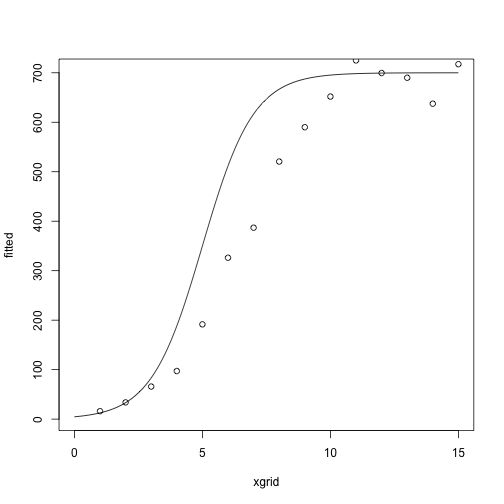
So far

• Newton’s method

• Things that reduce to Newton’s method

Today: modifications of Newton’s method

• Fisher scoring (if you want to make sure the Hessian term is negative definite)

• Hessian approximations (if it takes too long to re-compute/re-invert the Hessian)

• Gradient descent (if you don’t want to ever compute or invert the Hessian)

Reading:

• Boyd and Vandenberghe, Chapter 9.1-9.4

• Kenneth Lange, Numerical Analysis for Statisticians, Sections 13.3-13.6

Fisher Scoring

Idea: Use the expected information, \(I(\theta)= E[-d^2 \ell(\theta)]\) instead of the observed information, \(d^2 \ell(\theta)\).

Algorithm:

• Pick a starting parameter estimate \(\theta_0\)

• Set \(\theta_{n+1} = \theta_n + I(\theta)^{-1} d\ell(\theta_n)\)

Example: Non-linear least squares

Inputs:

• Data \(y_1,\ldots, y_n\).

• Covariates \(x_1,\ldots, x_n\).

• Parameter vector \(\theta\)

• Non-linear function \(\mu\), with \(\mu(x, \theta_1, \theta_2, \theta_3) = \frac{\theta_3}{1 + e^{-\theta_1 + \theta_2 x}}\)

• For notational purposes, let \(\mu_i (\theta) = \mu(x_i, \theta_1,\theta_2,\theta_3)\).

Model: \[ y_i \sim N(\mu_i(\theta), \sigma^2) \]

Log likelihood: \[ \ell(\theta) = - \frac{1}{2} \sum_{i=1}^n (y_i - \mu_i(\theta))^2 + C \]

Gradient/score: \[ \begin{align*} d\ell(\theta) &= \sum_{i=1}^n (y_i - \mu_i(\theta)) d\mu_i(\theta)\\ d\mu_i(\theta) &= \begin{pmatrix} \frac{\theta_3 e^{-\theta_1 - \theta_2 x}}{(1 + e^{-\theta_1 - \theta_2 x})^2} \\ \frac{x\theta_3 e^{-\theta_1 - \theta_2 x}}{(1 + e^{-\theta_1 - \theta_2 x})^2} \\ \frac{1}{(1 + e^{-\theta_1 - \theta_2 x})^2} \end{pmatrix} \end{align*} \]

Hessian: \[ d^2 \ell(\theta) = -\sum_{i=1}^n d \mu_i(\theta) d \mu_i(\theta)^T + \sum_{i=1}^n (y_i - \mu_i(\theta))d^2 \mu_i(\theta) \]

Information: \[ I(\theta) = E[-d^2 \ell(\theta)] = \sum_{i=1}^n d\mu_i(\theta) d\mu_i(\theta)^T \]

Example

fisher_scoring_iterate = function(x, y, theta_current) {
    score = compute_score(x, y, theta_current)
    information = compute_information(x, theta_current)
    theta_new = theta_current + solve(information) %*% score
}
compute_score = function(x, y, theta) {
    fitted = nonlin_function(x, theta)
    grad_mu = compute_grad_mu(x, theta)
    rowSums(sweep(grad_mu, 2, STATS = y - fitted, FUN = "*"))
}
compute_information = function(x, theta) {
    ## a 3 x n matrix
    grad_mu = compute_grad_mu(x, theta)
    grad_mu %*% t(grad_mu)
}
compute_grad_mu = function(x, theta) {
    denom = 1 + exp(-theta[1] - theta[2] * x)
    g1 = theta[3] * exp(-theta[1] - theta[2] * x) / denom^2
    g2 = x * theta[3] * exp(-theta[1] - theta[2] * x) / denom^2
    g3 = 1 / denom
    return(rbind(g1, g2, g3))
}
nonlin_function = function(x, theta) {
    theta[3] / (1 + exp(-theta[1] - theta[2] * x))
}

At the starting values:

library(NISTnls)
data(Ratkowsky3)
x = Ratkowsky3$x
y = Ratkowsky3$y
theta = c(-5, 1, 700)
xgrid = seq(0, 15, length.out = 1000)
fitted = nonlin_function(xgrid, theta)
plot(fitted ~ xgrid, type = 'l')
points(y ~ x)

After one iteration:

(theta = fisher_scoring_iterate(x, y, theta))

##           [,1]
## g1  -3.3298463
## g2   0.4649027
## g3 677.8340519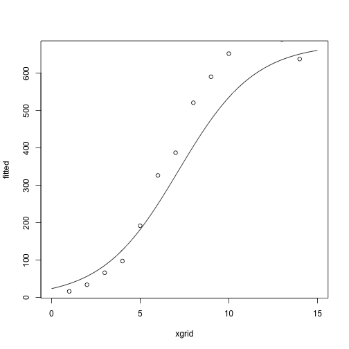

fitted = nonlin_function(xgrid, theta)
plot(fitted ~ xgrid, type = 'l')
points(y ~ x)

After two iterations:

(theta = fisher_scoring_iterate(x, y, theta))

##           [,1]
## g1  -4.2780124
## g2   0.6775608
## g3 664.2494602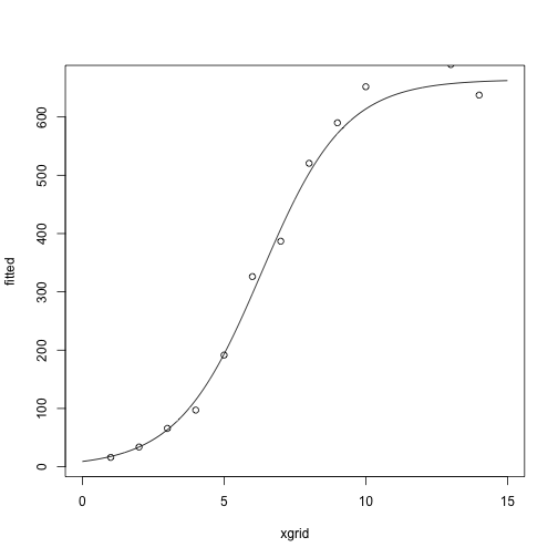

fitted = nonlin_function(xgrid, theta)
plot(fitted ~ xgrid, type = 'l')
points(y ~ x)

After several more iterations

for(i in 1:5) {
    theta = fisher_scoring_iterate(x, y, theta)
    print(theta)
}

##          [,1]
## g1  -4.438590
## g2   0.687286
## g3 702.939738
##           [,1]
## g1  -4.4435690
## g2   0.6887401
## g3 702.8457366
##           [,1]
## g1  -4.4424684
## g2   0.6885486
## g3 702.8741477
##           [,1]
## g1  -4.4425736
## g2   0.6885677
## g3 702.8711538
##           [,1]
## g1  -4.4425628
## g2   0.6885657
## g3 702.8714589

Compare with

nls(y ~ b3 / ((1+exp(-b1-b2*x))), data = Ratkowsky3,
    start = c(b1 = -5, b2 = 0.75, b3 = 700),
    trace = TRUE)

## 12935.59 :   -5.00   0.75 700.00
## 8971.367 :   -4.3638666   0.6765795 703.9695386
## 8930.131 :   -4.4470558   0.6894499 702.6779778
## 8929.885 :   -4.4420175   0.6884684 702.8858827
## 8929.883 :   -4.4426184   0.6885758 702.8698817
## 8929.883 :   -4.4425582   0.6885649 702.8715881

## Nonlinear regression model
##   model: y ~ b3/((1 + exp(-b1 - b2 * x)))
##    data: Ratkowsky3
##       b1       b2       b3 
##  -4.4426   0.6886 702.8716 
##  residual sum-of-squares: 8930
## 
## Number of iterations to convergence: 5 
## Achieved convergence tolerance: 5.737e-06

Quasi-Newton Methods

Idea: If you don’t move very far in one step, the Hessian shouldn’t change that much either.

Instead of recomputing the Hessian at each step, compute an approximate update.

• Start with an initial guess at a parameter \(\theta^{(0)}\).

• Let \(A^{(0)} = d^2 \ell(\theta)\).

• Set \(\theta^{(n+1)} = \theta^{(n)} - (A^{(n)})^{-1} d \ell(\theta^{(n)})\)

• Set \(A^{(n+1)} = A^{(n)} - c^{(n)} v^{(n)} (v^{(n)})^T\)

\(A^{(n)}\) are approximations to the Hessian.

Idea behind Hessian update: Taylor series again:

\[ d\ell(\theta^{(n)}) \approx d\ell(\theta^{(n+1)}) + d^2 \ell(\theta^{(n+1)})(\theta^{(n)} - \theta^{(n+1)}) \]

For notation, let \[ \begin{align*} g^{(n)} &= d\ell(\theta^{(n)}) - d \ell(\theta^{(n+1)}) \\ s^{(n)} &= \theta^{(n)} - \theta^{(n+1)} \end{align*} \]

We can rewrite the secant condition \[ d\ell(\theta^{(n)}) - d\ell(\theta^{(n+1)})\approx d^2 \ell(\theta^{(n+1)})(\theta^{(n)} - \theta^{(n+1)}) \] as \[ -A^{(n+1)} s^{(n)} = g^{(n)} \]

Davidson’s method is a symmetric rank-1 update.

\[ A^{(n+1)} = A^{(n)} - c^{(n)} v^{(n)} (v^{(n)})^T \]

where \[ c^{(n)} = \frac{1}{(g^{(n)} + A^{(n)} s^{(n)})^T s^{(n)}} \\ v^{(n)} = g^{(n)} + A^{(n)} s^{(n)} \]

(verify on your own that this satisfies the secant condition)

BFGS is a symmetric rank-2 update.

\[ A^{(n+1)} = A^{(n)} + \alpha u u^T + \beta v v^T \]

\(u = y^{(k)}\), \(v = A^{(n)} s^{(n)}\), \(\alpha = -1 / (g^{(k)})^T s^{(k)}\), \(\beta = - 1 / (s^{(k)})^T B^{(k)} s^{(k)}\)

Why are these useful?

• This makes it easy to compute an approximation of \(-d^2 \ell(\theta)\), but we still need to invert it to take an approximate Newton step

• Woodbury matrix identity allows us to compute the inverse of a low-rank update quickly

\[ (A + UCV)^{-1}= A^{-1} - A^{-1} U(C^{-1} + VA^{-1} U)^{-1} V A^{-1} \]

Gradient descent

Our problem:

\[ \text{minimize}_x \quad f(x) \]

Note that we’re doing minimization instead of maximization now so that the notation matches the reading, but any minimization problem can be recast as a maximization and vice versa.

Descent Methods

General algorithm:

Start with a point \(x\)

Repeat

• Choose a descent direction \(\Delta x\)

• Choose step size \(t\).

• Update: \(x \leftarrow x + t \Delta x\)

Until the stopping criterion is satisfied, usually \(\|\nabla f(x)\|_2 \le \epsilon\).

Line search types: Exact line search

Step size \(t\) found as \[ t = \text{argmin}_{t > 0}f(x + t \Delta x) \]

This can be useful if there is an analytic or otherwise quick method of finding the minimum of the function restricted to a ray.

Line search types: Backtracking line search

• Step size \(t\) found with an iterative method.

• Parameters \(\alpha \in (0, 1/2)\), \(\beta \in (0,1)\) that you specify.

• Algorithm: Start at \(t = 1\), repeat \(t \leftarrow \beta t\) until \[ f(x + t \Delta x) < f(x) + \alpha t \nabla f(x)^T \Delta x \]

Gradient descent

In gradient descent, we take \(\Delta x = - \nabla f(x)\).

Overall algorithm:

Start with a point \(x\)

Repeat

• \(\Delta x \leftarrow - \nabla f(x)\).

• Line search: Choose step size \(t\) by either backtracking line search or exact line search.

• Update: \(x \leftarrow x + t \Delta x\)

Until the stopping criterion is satisfied, usually \(\|\nabla f(x)\|_2 \le \epsilon\).

Gradient descent example

Iterates of gradient descent with backtracking line search, for minimizing \(f(x_1, x_2) = \exp(x_1 + 3 x_2 - .1) + \exp(x_1 - 3 x_2 - .1) + \exp(-x_1 - .1)\)

Contours represent the boundaries of the sublevel sets of the function: \(\{x : f(x) \le a\}\).

Steepest descent

Steepest descent: modification of the descent direction.

The normalized steepest descent direction is defined as \[ \Delta x_{nsd} = \text{argmin}_x \{\nabla f(x)^T v : \|v\| = 1\} \] for some norm \(\|\cdot \|\).

Note: Steepest descent with the standard norm (\(\|\cdot\|_2\)) is the same as gradient descent.

Steepest descent algorithm

The same as gradient descent, but with a different descent direction:

Start with a point \(x\)

Repeat

• \(\Delta x \leftarrow \Delta x_{sd}\).

• Line search: Choose step size \(t\) by either backtracking line search or exact line search.

• Update: \(x \leftarrow x + t \Delta x_{sd}\)

Until the stopping criterion is satisfied, usually \(\|\nabla f(x)\|_2 \le \epsilon\).

Normalized steepest descent direction for a quadratic norm

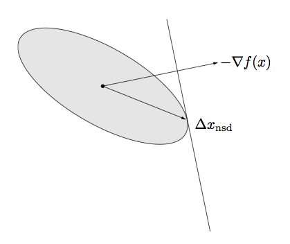
• Ellipse is the set \(\{v: \|v\|_P \le 1\}\)

• \(\Delta x_{nsd}\) is the point in the ellipse that extends farthest in the direction of \(-\nabla f(x)\).

• Analytic solution for the steepest descent direction: \[ \Delta x_{nsd} = -(\nabla f(x)^T P^{-1} \nabla f(x))^{-1/2} P^{-1} \nabla f(x) \]

• There is a standard way of normalizing, involving a dual norm (see the text if you’re interested), the unnormalized steepest descent search direction is \[ \Delta x_{sd}= -P^{-1} \nabla f(x) \]

Examples of the effect of the norm

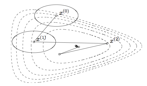
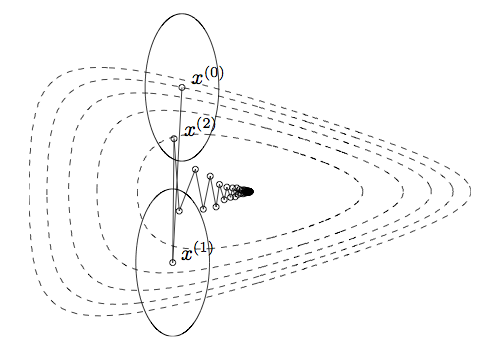
• The choice of norm changes dramatically the number of steps needed to reach the optimum

• Steps show steepest descent/backtracking line search for quadratic norms

• Ellipses are the norm balls around each of the iterates

When can we expect these methods to do well?

From the pictures, we saw that

• Gradient descent doesn’t do well when the sublevel sets are far from spherical

• Steepest descent does well when the norm balls approximate the sub-level sets.

Quadratic norms as a gradient descent in a transformed coordinate system

The quadratic norm \(\|\cdot\|_P\) is defined as \(\|x\|_P = x^T P x\), where \(P\) is a positive definite matrix.

Steepest descent with the \(\|\cdot\|_P\) norm is the same as gradient descent after a change of coordinates:

• Let \(\bar u = P^{1/2} u\)

• \(\|u\|_P = \|\bar u\|_2\)

• \(\bar f(\bar u) = f(P^{-1/2} \bar u) = f(u)\)

• Applying gradient descent to \(\bar f\) is equivalent to applying steepest descent with the \(\|\cdot\|_P\) norm to \(f\).

For example

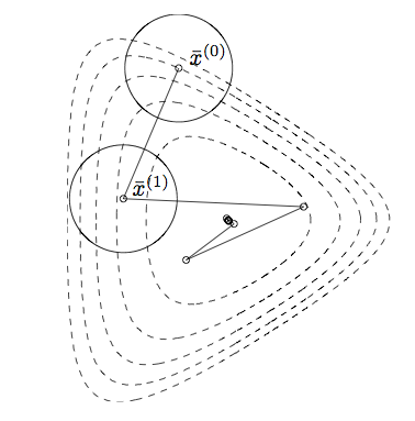
• Gradient descent on a transformed version of the problem before.

• Sublevel sets now much closer to spherical, and the algorithm converges quickly.

Convergence theorem

Suppose \(f\) is strongly convex, so that there are constants \(m\) and \(M\) such that \(mI \preceq d^2 f \preceq MI\).

Let \(x^{(k)}\) be the solution after \(k\) steps of gradient descent with exact line search, and let \(p^\star\) be the minimizing value of \(f\).

Then \[ f(x^{(k)}) - p^\star \le (1 - m/M)^k (f(x^{(0)}) - p^\star) \]

(Equation 9.18 in Boyd and Vandenberghe)

Re-interpretation of Newton’s method

• Recall the Newton step: \(-\nabla^2 f(x)^{-1} \nabla f(x)\)

• This search direction is the same as the steepest descent direction in the Hessian norm: \(\|\cdot\|_{\nabla^2 f(x)}\)

• Turns out the Hessian norm gives a good approximation of the contours of the sublevel sets around the optimal point: this is why it has such fast convergence.

Summing up

• Everything we’ve seen has an interpretation as Newton’s method with some approximation of the Hessian standing in for the real thing

• Everything we’ve seen has an interpretation as gradient descent in a transformed coordinate system

• You need to trade off between using the analytic information you have about the problem and computational complexity.