Git: local and remote repositories
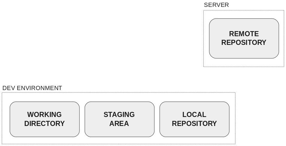
When using github, you have two repositories: the one on your computer, and the one on the server.
Logistics:
New homework posted
Extend deadline for this homework to Friday
Agenda today
Newton’s method for multivariate problems
Generalized linear models and exponential familiies
Iteratively reweighted least squares for maximum likelihood in generalized linear models
Remote repositories for git/github
Reading:
Newton’s method:
Pick some starting value \(\theta^{(0)}\)
Iterate: \(\theta^{(m+1)} = \theta^{(m)} - d^2 \ell(\theta^{(m)}) d \ell(\theta^{(m)})\)
Stop when \(d\ell(\theta^{(m)})\) is sufficiently close to 0.
Linear regression model:
Likelihood: \[ L(\theta) = (2\pi)^{-n/2} \sigma^{-n}\exp(-(y - X\theta)^T (y - X\theta) / 2) \]
Log likelihood: \[ \ell(\theta) = -n \log(2\pi) / 2 - n \log \sigma - (y - X \theta)^T (y - X \theta) / 2 \]
\(d\ell(\theta)\): \[ X^T (y - X \theta) \]
\(d^2 \ell(\theta)\): \[ -X^T X \]
Newton step: \[ \begin{align*} \theta^{(1)} &= \theta^{(0)} - d^2 \ell(\theta^{(0)})^{-1} d \ell(\theta^{(0)})\\ &= \theta^{(0)} - (-X^T X)^{-1} X^T(y - X \theta^{(0)}) \\ &= \theta^{(0)} + (X^T X)^{-1} X^T y - (X^T X)^{-1} X^T X \theta^{(0)} \\ &= (X^T X)^{-1} X^T y \end{align*} \]
Logistic regression model:
Likelihood: \[ L(\theta) = \prod_{i=1}^n p_i^{y_i} (1 - p_i)^{1 - y_i} \]
Log likelihood: \[ \begin{align*} \ell(\theta)&= \sum_{i=1}^n (y_i \log p_i + (1 - y_i) \log(1 - p_i)) \\ &= \sum_{i=1}^n (y_i x_i^T \theta - \log(1 + \exp(x_i^T \theta))) \end{align*} \]
First derivatives: \[ \begin{align*} d\ell(\theta) &= \sum_{i=1}^n \left(y_i x_i - \frac{\exp(x_i^T \theta)}{1 + \exp(x_i^T \theta)} x_i\right) \\ &= \sum_{i=1}^n (y_i - p_i) x_i \\ &= X^T (y - p) \end{align*} \]
Second derivatives: \[ \begin{align*} d^2 \ell(\theta) &= \sum_{i=1}^n p_i(1 - p_i) x_i x_i^T \\ &= -X^T W X \end{align*} \] if \(W = \text{diag}(p_1(1 - p_1), \ldots, p_n(1 - p_n))\)
Newton step: \[ \begin{align*} \theta^{(m+1)} &= \theta^{(m)} - (d^2 \ell(\theta))^{-1} d \ell(\theta) \\ &= \theta^{(m)} + (X^T W^{(m)} X)^{-1} X^T (y - p^{(m)}) \end{align*} \]
Exponential families are families of probability distributions whose densities take the form \[ f(x | \eta) = h(x) exp(\eta^T T(x) - A(\eta)) \]
\(T\) and \(A\) are known functions that describe the family.
\(\eta\) is the natural parameter.
Properties that we’ll need later:
\(E(X) = A'(\eta)\)
\(\text{var}(X)= A''(\eta)\)
Why do we like them?
Many commonly-used distributions: normal, exponential, Poisson, binomial, multinomial, etc.
Easy to analyze
They describe the stochasticity in generalized linear models
Models for independent observations, \(y_i, i = 1,\ldots, n\)
Three components:
The canonical link is the one that maps the mean to the natural parameter.
Normal: Canonical link is the identity: \(g(x) = x\)
Bernoulli: Canonical link is logit: \(g(x) = \log(x / (1 - x))\)
Poisson: Canonical link is the log: \(g(x) = \log(x)\)
Gamma: Canonical link is inverse: \(g(x) = x^{-1}\)
Find \(\eta_i^{(m)} = x_i^T \theta^{(m)}\), \(i = 1,\ldots, n\)
Find \(\mu_i^{(m)} = g^{-1} (\eta_i^{(m)})\)
Idea:
The problem is linear in the natural parameter space, so try to do least squares there
“Working dependent variable” is like \(y_i\) mapped to the natural parameter space.
In general, a random variable taken from an exponential family distribution will have variance that depends on the natural parameter.
The weights are inversely proportional to the variance of the response at the current guess for \(\theta\).
Samples for which the variance should be smaller have larger weights, samples for which the variance should be larger get smaller weights
Random component: normal distribution, \(y_i \sim N(\eta_i, 1)\) (variance 1 for ease of notation, everything goes through analogously with unknown variance \(\sigma\))
Exponential family representation of the normal distribution has \(A(\eta) = \eta^2 / 2\)
Systematic component: \(\eta_i = x_i^T \theta\)
Canonical link function for the normal distribution is \(g(x) = x\), so \(\eta_i = \mu_i\)
Identity link means \(E(y_i) = g^{-1}(\eta_i) = g^{-1}(x_i^T \theta) = x_i^T \theta\)
Working dependent variable at iteration \(0\) \[ \begin{align*} z_i^{(0)} &= \eta_i^{(0)} + (y_i - \mu_i^{(0)}) d \eta_i^{(0)}/ d\mu\\ &= \mu_i^{(0)} + (y _i - \mu_i^{(0)}) = y_i \end{align*} \]
Iterative weights: \[ \begin{align*} w_i^{(0)} &= (A''(\eta_i^{(0)}) d\eta_i^{(0)} / d\mu)^{-1} \\ &= 1 \end{align*} \]
New estimate is \[ \begin{align*} \theta^{(1)} &= (X^T W^{(0)} X)^{-1} X^T W^{(0)} z\\ &= (X^T X)^{-1} X^T y \end{align*} \]
Random component: Bernoulli distribution, \(y_i \sim \text{Bernoulli}(\mu_i)\), \(\mu_i \in (0,1)\)
Systematic component: \(\eta_i = x_i^T \theta\)
Canonical link for Bernoulli is \(g(x) = \log(x / (1 - x))\), so \(\eta_i = \log(\mu_i / (1 - \mu_i))\)
Exponential family representation of Bernoulli has \(A(\eta) = \log (1 + e^\eta)\)
Quantities we will need: \[ \eta = \log (\mu / (1 - \mu)) \]
\[ d\eta / d\mu = 1/\mu + 1 / (1 - \mu) = 1 / (\mu(1 - \mu)) \]
\[ A(\eta) = \log(1 + e^\eta) \]
\[ A'(\eta) = \frac{e^\eta}{1 + e^\eta} \]
\[ \begin{align*} A''(\eta) &= \frac{e^\eta}{(1 + e^\eta)^2}\\ &= \mu(1 - \mu) \end{align*} \]
Working dependent variables: \[ z_i = \eta_i + (y_i - \mu_i) \frac{d\eta_i}{d \mu_i}\\ = \eta_i + \frac{y_i - \mu_i}{\mu_i(1 - \mu_i)} \]
Iterative weights: \[ \begin{align*} w_i &= (A''(\eta_i) (\frac{d\eta_i}{d\mu_i})^2)^{-1} \\ &= (\mu_i(1 - \mu_i) (\mu_i(1 - \mu_i))^{-2})^{-1}\\ &= \mu_i(1 - \mu_i) \end{align*} \]
Update formula:
\[ \theta^{(m+1)} = (X^T W^{(m)} X)^{-1} X^T W^{(m)} z^{(m)} \]
Notice that we can rewrite this: \[ \begin{align*} \theta^{(m+1)} &= (X^T W^{(m)} X)^{-1} X^T W^{(m)} z^{(m)} \\ &= (X^T W^{(m)} X)^{-1} X^T W^{(m)} (\eta^{(m)} + \frac{y^{(m)} - \mu^{(m)}}{\mu^{(w)}(1 - \mu^{(m)})}) \\ &= (X^T W^{(m)} X)^{-1} X^T W^{(m)} (X\theta^{(m)} + (W^{(m)})^{-1}(y - \mu^{(m)}))\\ &= \theta^{(m)} + (X^T W^{(m)} X)^{-1} X^T (y - \mu^{(m)}) \end{align*} \]
Remember Newton-Raphson for logistic regression?
Different from Newton-Raphson if you use a non-canonical link
One example: probit regression instead of logistic regression
Interpretation of Newton-Raphson suggests algorithms for other models

When using github, you have two repositories: the one on your computer, and the one on the server.
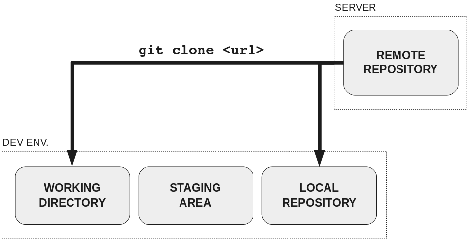
Data from the remote repository is put in your working directory and local repository.
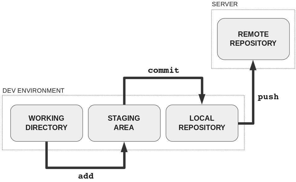
You make changes locally using git add and git commit
You can upload your local commits to the remote repository using `git push
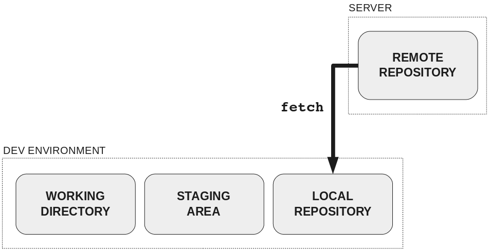
You can use git fetch, but that will only add the new commits to your repository, it won’t change your working directory.
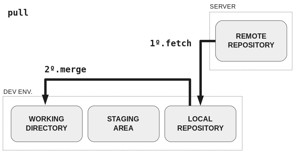
git pull is like git fetch + git merge: it fetches the new commits and then updates your working directory to correspond with the most recent commits from the server.
Note: all the pictures from Rachel Carmena, some good resources at that website.