adaptiveGPCA

Description

Adaptive gPCA, described in Fukuyama (2017), is a flexible method for incorporating information about the relationships between the variables into principal components analysis. It was developed for incorporating information about the phylogenetic structure of bacteria in microbiome data analysis, but it is applicable more generally (for example, graph structure on the variables or distances between the variables).

Installation

The method is implemented in the R package adaptiveGPCA. To install, use

install.packages("adaptiveGPCA")

Quick start for microbiome data

The package comes with a full vignette, which explains all of the functions and their arguments. To get a feel for what the package does, you can try out the following commands, which run adaptive gPCA on an example microbiome dataset that comes with the package.

First we load the required packages

library(adaptiveGPCA)
library(ggplot2)
library(phyloseq)

Then load the example data, which is stored as a phyloseq object, and process it to get the correct input for adaptive gPCA.

data(AntibioticPhyloseq)
pp = processPhyloseq(AntibioticPhyloseq)

The next command creates a sequence of ordinations with a range of values for the structure parameter, going from no structure to maximal structure. The visualizeFullFamily function will open a browser window and allows you to see the effect of changing this parameter interactively.

out.ff = gpcaFullFamily(pp$X, pp$Q, k = 2)
out.agpca = visualizeFullFamily(out.ff,
    sample_data = sample_data(AntibioticPhyloseq),
    sample_mapping = aes(x = Axis1, y = Axis2, color = type),
    var_data = tax_table(AntibioticPhyloseq),
    var_mapping = aes(x = Axis1, y = Axis2, color = Phylum))

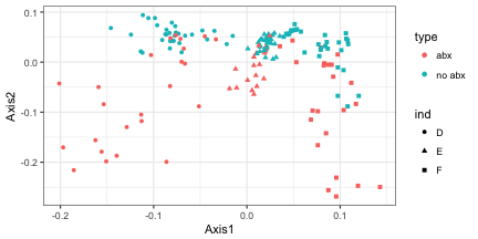
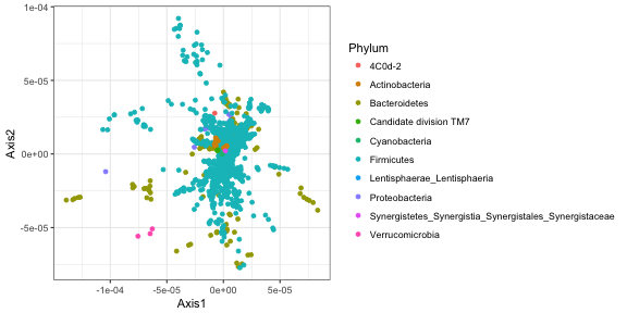
The adaptivegpca function chooses the structure parameter automatically, and we can make plots of the samples and species corresponding to that value of the structure parameter.

out.agpca = adaptivegpca(pp$X, pp$Q, k = 2)
ggplot(data.frame(out.agpca$U, sample_data(AntibioticPhyloseq))) +
    geom_point(aes(x = Axis1, y = Axis2, color = type, shape = ind))

ggplot(data.frame(out.agpca$QV, tax_table(AntibioticPhyloseq))) +
    geom_point(aes(x = Axis1, y = Axis2, color = Phylum))

Finally, the inspectTaxonomy function will open a browser window that allows you to get more information about the taxa in the plot above.

t = inspectTaxonomy(out.agpca, AntibioticPhyloseq)